Annotated PID Controller in SWMM5 and InfoSWMM

How does a PID controller work in  InfoSWMM  and SWMMM 5 - this also applies to H2OMap SWMM??

double getPIDSetting(struct TAction* a, double dt)   //  at each time  step find  the PID control  changes for the  current  time step dt
// Input: a = an action object
// dt = current time step (days)
// Output: returns a new link setting
// Purpose: computes a new setting for a link subject to a PID controller.

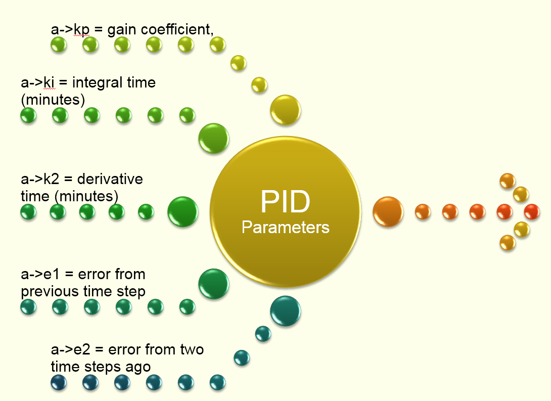
// Note: a->kp = gain coefficient,
// a->ki = integral time (minutes)
// a->k2 = derivative time (minutes)
// a->e1 = error from previous time step
// a->e2 = error from two time steps ago
{
double e0, setting;
double p, i, d, update;
double tolerance = 0.0001;

// --- convert time step from days to minutes
dt *= 1440.0;

// --- determine relative error in achieving controller set point

// Or how close are we to the set point?

e0 = SetPoint - ControlValue;
if ( fabs(e0) > TINY )
{
if ( SetPoint != 0.0 ) e0 = e0/SetPoint;

// now alter the  value of e0

else e0 = e0/ControlValue;
}

// --- reset previous errors to 0 if controller gets stuck
if (fabs(e0 - a->e1) < tolerance)
{
a->e2 = 0.0;
a->e1 = 0.0;
}

// --- use the recursive form of the PID controller equation to
// determine the new setting for the controlled link

Here is a view of the p, i and d PID internal  parameters https://www.wikiwand.com/en/PID_controller

A block diagram of a PID controller in a feedback loop

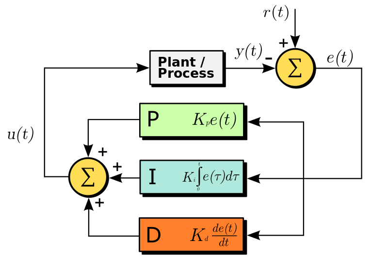
p = (e0 - a->e1);

ki, id,  kp are  user  inputs  in InfoSWMM and SWMM5 or from the  EPA SWMM  5 Help  File

if ( a->ki == 0.0 ) i = 0.0;
else i = e0 * dt / a->ki;

d = a->kd * (e0 - 2.0*a->e1 + a->e2) / dt;

update = a->kp * (p + i + d);
if ( fabs(update) < tolerance ) update = 0.0;
setting = Link[a->link].targetSetting + update;

// --- update previous errors
a->e2 = a->e1;
a->e1 = e0;

// --- check that new setting lies within feasible limits

// If  the link  is not a pump then the  setting must be between 0 and 1
if ( setting < 0.0 ) setting = 0.0;
if (Link[a->link].type != PUMP && setting > 1.0 ) setting = 1.0;
return setting;}

InfoSWMM 2D Version 13 Brings Significant 1D and 2D Simulation Advancements To Power Users

Latest Release Confirms Product as Leading GIS-centric Urban Drainage Modeling and Management Solution

Broomfield, Colorado, USA, November 18, 2014

Innovyze, a leading global innovator of business analytics software and technologies for smart wet infrastructure, today announced the worldwide availability of the V13 Generation of its industry-leading InfoSWMM 2D for ArcGIS (Esri, Redlands, CA). InfoSWMM 2D delivers new ways to quickly and accurately build and analyze very large and comprehensive two-dimensional (2D) models that reliably simulate complex urban stormwater, sanitary sewers, river flooding and pollutant transport. It allows users to accurately predict the extent and duration of urban and rural flooding for comprehensive stormwater management directly within the powerful ArcGIS environment.

A fully hydrodynamic geospatial stormwater modeling and management software application, InfoSWMM 2D can be used to model the entire land phase of the hydrologic cycle as applied to urban stormwater systems. Built atop ArcGIS and using exceptionally robust and efficient numerical simulation capabilities, the model can perform single-event or long-term (continuous) rainfall/runoff simulations accounting for climate, soil, land use, and topographic conditions of the watershed. In addition to simulating runoff quantity, InfoSWMM 2D can reliably predict runoff quality, including buildup and washoff of pollutants from primarily urban watersheds. It also features very sophisticated Real-Time Control (RTC) schemes for the operational control and management of hydraulic structures.

A hallmark of InfoSWMM 2D is its dynamic integration of one-dimensional (1D) hydrodynamic simulation of flows in open channels, HEC-22 inlets and closed pipe networks with two-dimensional (2D) hydrodynamic simulation of surface runoff, evaporation, infiltration and flooding in the urban environment. The dynamic integration, achieved through an explicit coupling of 1D and 2D flow equations, provides a powerful solution for simultaneously modeling belowground and aboveground elements of watersheds to accurately represent all flow paths and improve understanding of holistic processes. InfoSWMM 2D also directly simulates the rainfall and infiltration on both the watershed and the 2D surface to better simulate 1D flooding, 2D surface flooding, 2D shallow groundwater recharge and complex 1D and 2D surface interactions.

The full 2D free-surface shallow water equations are solved using a highly advanced finite volume method, which is particularly suitable for rapidly varying flood flows such as those moving through steep streets and road junctions and those associated with bank overtopping or breaching. The unparalleled 1D/2D dynamic linking capabilities of InfoSWMM 2D give engineers the unprecedented power to analyze and predict potential flood extents, depth and velocity and accurately model the interaction of surface and underground systems in an integrated 1D/2D environment. The software can be used to simulate point sources, 2D boundaries, multiple 2D mesh and simulation polygons in a sewer or stormwater network. The combined water level and velocity results throughout the flooded areas can be viewed as various comprehensive graphs; tables; or animated, thematic flood maps.

Among its many new enhancements, Version 13 uses a significantly improved 2D simulation engine, the flexible InfoSWMM ArcMap polygon tools, a 1D InfoSWMM engine based on the latest EPA SWMM 5.1, a new 1D and 2D graphics engine and a comprehensive Output Report Manager and Statistical Event Manager for both 1D and 2D output. In addition, the new release allows users to instantly visualize the maximum extent of flooding in vivid 2D and 3D maps.

“We’re deeply committed to providing a geospatial modeling experience that is both intuitive and powerful, and InfoSWMM 2D V13 embodies that commitment,” said Paul F. Boulos, Ph.D., BCEEM, NAE, Hon.D.WRE, Dist.D.NE, F.ASCE, President, COO and Chief Technical Officer of Innovyze. “This release delivers major geotechnological and computational enhancements in short release cycles to make sure our customers are always equipped with the ultimate ArcGIS-centric decision support tool for stormwater and urban drainage systems. It greatly extends the core features of InfoSWMM, providing the most powerful and comprehensive ArcGIS-centric tool kit ever for managing the risks of urban and rural flooding. This is a must have for effectively controlling and managing sanitary sewer and combined sewer overflows.”

How to Set a Flap Gate in InfoSWMM

Note:  How to Set a Flap Gate in InfoSWMM

You can set a flap gate in InfoSWMM either by using the attribute browser and changing the Flap Gate Installed to Yes or No or by using the DB Editor and changing the Flag for Flap Gate Installed to Yes by using the Block Edit tool.   The DB method is better for changing many conduits. 

How Does a TYPE1 Pump Work in SWMM 5?

Subject:   How Does a TYPE1 Pump Work in SWMM 5?

A SWMM 5 Type1 pump is called an offline pump but the name comes from SWMM 4 and the Pump is controlled by volume instead of depth or head as in the SWMM 5 TYPE2, TYPE3 and TYPE4 Pumps.  The attached example SWMM 5 model has an offline storage node that pumps flow INTO the Offline Storage unit during high flow and FROM the Offline Storage Unit during low flow.  The SWMM 5 Real Time Control (RTC) rules determine which of the two pumps operate based on the flow in an upstream link (Figure 1). 

Figure 1.   RTC Rules and Schematic of an OffLine Pump in SWMM 5.

How is the Orifice Setting Used in SWMM 5 RTC Rules?

Subject:  How is the Orifice Setting Used in SWMM 5 RTC Rules?

The Real Time Control Rule for Orifice Setting can be a function of a Setting constant, Setting from a Curve, Setting from a PID controller and a Setting from a Time Series (Figure 1).    The Setting affects the Full Depth of the Orifice at each time step.  The setting which ranges from 0 to 1 can either completely close or open theorifice (Figure 2).   You will have to use the equivalent in ICM or else the settings derived from the SWMM 5 time series need to be multiplied by the orifice depth to have the same effect in ICM that it had in SWMM 5. 

Figure 1.  The Possibilities for defining the Setting of an Orifice in SWMM 5 from a H2OMAP SWMM RTC dialog.

 

 Figure 2.  The Setting affects the Full Depth of the Orifice at each time step.  The setting which ranges from 0 to 1 can either completely close or open the orifice.

SWMM 5 Weir RTC Rules

Subject:   SWMM 5 Weir RTC Rules

This example SWMM 5 model closes a weir based on the depth at the upstream node of the Weir every 0.25 feet.  You can see the effect of the RTC rules using a Scatter plot of Weir Flow versus Weir Depth in SWMM 5 (Figure 1).   The Weir flows normally every 0.25 feet but shuts down three times using these rules which set the Weir Setting to 0.0

RULE Weir100

IF Node  WeirNode Depth > 1.75

AND Node WeirNode Depth < 2.0

THEN WEIR WEIR Setting = 0.0

Priority 2

RULE Weir101

IF Node  WeirNode Depth > 2.25

AND Node WeirNode Depth < 2.5

THEN WEIR WEIR Setting = 0.0

Priority 2

RULE Weir102

IF Node  WeirNode Depth > 2.75

AND Node WeirNode Depth < 3.0

THEN WEIR WEIR Setting = 0.0

Priority 2

RULE Weir103

IF Node  WeirNode Depth > 3.25

AND Node WeirNode Depth < 3.5

THEN WEIR WEIR Setting = 0.0

Priority 2

RULE Weir104

IF Node  WeirNode Depth > 3.75

AND Node WeirNode Depth < 4.0

THEN WEIR WEIR Setting = 0.0

Priority 2

Figure 1.  Scatter Graph of Weir flow versus Weir Node Depth.

How to Approximate a Timer in the RTC Rules of SWMM 5

Subject:   How to Approximate a Timer in the RTC Rules of SWMM 5

SWMM 5 does not have a explicit timer in its Real Time Control (RTC) rules but you can approximate it by using a Control Curve as in the attached example model.  The Control Curve will modify the setting of the Weir by the Inflow to the Storage node.  You can have normal weir flow settings based on the invert elevation of the weir and the Surface node water surface elevation but in addition you can control the weir setting by:

1.   Closing the weir when the inflow is low,
2.   Closing the weir by staggered Storage node depth,
3.   Opening the weir gradually when the inflow increases
4.   Closing the weir by a combination of Node Depth IF statements and Control Curve rules

For example, you can have the Weir Setting controlled the Node Depth,  Link Inflow and Node Inflow  simultaneously approximately with the depth and the inflow parameters closing the weir by proxy instead of by time since the closing.

SWMM 5 Clocktime RTC Rules for Pumps, Weirs and Orifices

Subject:  SWMM 5 Clocktime RTC Rules for Pumps, Weirs and Orifices

You can use the Control or RTC rules in SWMM 5 to adjust the settings of the weirs, pumps and orifices based on the clock time each day of your simulation.  Here is an example that will adjust orifice height every ½ hour for 7 orifices at one time using two sets of rules.

RULE R1a 

; Half hour setting

IF SIMULATION CLOCKTIME = 0:30:00 

OR SIMULATION CLOCKTIME = 1:30:00  

OR SIMULATION CLOCKTIME = 2:30:00 

OR SIMULATION CLOCKTIME = 3:30:00 

OR SIMULATION CLOCKTIME = 4:30:00 

OR SIMULATION CLOCKTIME = 5:30:00 

OR SIMULATION CLOCKTIME = 6:30:00 

OR SIMULATION CLOCKTIME = 7:30:00 

OR SIMULATION CLOCKTIME = 8:30:00 

OR SIMULATION CLOCKTIME = 9:30:00 

OR SIMULATION CLOCKTIME = 10:30:00

OR SIMULATION CLOCKTIME = 11:30:00

OR SIMULATION CLOCKTIME = 12:30:00 

OR SIMULATION CLOCKTIME = 13:30:00  

OR SIMULATION CLOCKTIME = 14:30:00 

OR SIMULATION CLOCKTIME = 15:30:00 

OR SIMULATION CLOCKTIME = 16:30:00  

OR SIMULATION CLOCKTIME = 17:30:00 

OR SIMULATION CLOCKTIME = 18:30:00 

OR SIMULATION CLOCKTIME = 19:30:00 

OR SIMULATION CLOCKTIME = 20:30:00 

OR SIMULATION CLOCKTIME = 21:30:00 

OR SIMULATION CLOCKTIME = 22:30:00

OR SIMULATION CLOCKTIME = 23:30:00

THEN ORIFICE R1 SETTING = 0.90

AND  ORIFICE R2 SETTING = 0.90

AND  ORIFICE R3 SETTING = 0.90

AND  ORIFICE R4 SETTING = 0.90

AND  ORIFICE R5 SETTING = 0.90

AND  ORIFICE R6 SETTING = 0.90

AND  ORIFICE R7 SETTING = 0.90

RULE R1b

; hour setting

IF SIMULATION CLOCKTIME = 0:00:00

OR SIMULATION CLOCKTIME = 1:00:00

OR SIMULATION CLOCKTIME = 2:00:00

OR SIMULATION CLOCKTIME = 3:00:00

OR SIMULATION CLOCKTIME = 4:00:00

OR SIMULATION CLOCKTIME = 5:00:00

OR SIMULATION CLOCKTIME = 6:00:00

OR SIMULATION CLOCKTIME = 7:00:00

OR SIMULATION CLOCKTIME = 8:00:00

OR SIMULATION CLOCKTIME = 9:00:00

OR SIMULATION CLOCKTIME = 10:00:00

OR SIMULATION CLOCKTIME = 11:00:00

OR SIMULATION CLOCKTIME = 12:00:00 

OR SIMULATION CLOCKTIME = 13:00:00

OR SIMULATION CLOCKTIME = 14:00:00 

OR SIMULATION CLOCKTIME = 15:00:00

OR SIMULATION CLOCKTIME = 16:00:00

OR SIMULATION CLOCKTIME = 17:00:00

OR SIMULATION CLOCKTIME = 18:00:00 

OR SIMULATION CLOCKTIME = 19:00:00 

OR SIMULATION CLOCKTIME = 20:00:00 

OR SIMULATION CLOCKTIME = 21:00:00 

OR SIMULATION CLOCKTIME = 22:00:00 

OR SIMULATION CLOCKTIME = 23:00:00

THEN ORIFICE R1 SETTING = 0.5

AND  ORIFICE R2 SETTING = 0.5

AND  ORIFICE R3 SETTING = 0.5

AND  ORIFICE R4 SETTING = 0.5

AND  ORIFICE R5 SETTING = 0.5

AND  ORIFICE R6 SETTING = 0.5

AND  ORIFICE R7 SETTING = 0.5

How to see the effect of the Pump Setting in the RTC Rules of InfoSWMM and H20MAP SWMM

Subject:  How to see the effect of the Pump Setting in the RTC Rules of InfoSWMM and H20MAP SWMM

Step 1.   Pump Startup and Shutoff Depth

Depths to turn the Pump On and turn the Pump Off.  In this example, the pump will be off when the Wet Well Depth is less than 2 feet, the Pump will be off between a Wet Well Depth between 2 and 5.75 feet if the Pump is currently Off and the Pump will be On between a Wet Well Depth between 5.75 and 2 feet.

Step 2.   RTC Rule for the Pump Setting when the Wet Well Depth is less than 6.25 feet.  We need to add the AND statement so that the setting is only reset when the Pump is On.   You do not want the pump setting to be reset when the pump should be off.

Result 1:  The Pump Speed Ratio tells you the Pump Setting

Result 2:  RTC Control Rules in the RPT File if you click on Show Control Actions

Result 3:   The depth at the Wet Well and the Flow in the Pump

Result 4:  A mixed graph of the Wet Well Depth and Pump Flow shows the effect of the RTC.

Result 5:  The RTC Rule can also been seen flow to the Pump Curve.

Example RTC rule for the opening and closing of the orifice in SWMM5

Here is an example Real Time Control (RTC) rule for the opening and closing of  an orifice in SWMM5.

RULE Orifice1

IF SIMULATION  CLOCKTIME >=  01:00:00

AND SIMULATION CLOCKTIME <=  2:00:00

THEN ORIFICE OR1@82309b-15009b SETTING = 1

ELSE ORIFICE OR1@82309b-15009b SETTING = 0

PRIORITY 1

; Opens up the orifice at hour 1 of the simulation

Orifice Open and Close Speed and the Target Setting

Orifice Open and Close Speed and the Target Setting

In SWMM 5 there is an orifice parameter called setting which opens or closes the orifice opening by modifying the depth of the orifice.  The setting is  based either on a RTC rule of the orifice or the Flap Gate condition of the orifice and can be between 0 and 1.  Closed is 0; Open is 1.  The difference is that the target setting is what the setting should be based on the condition of the Flap Gate or the RTC Rules and the setting is the value actually used in the model. 

The open and close speed of the orifice modifies the orifice setting by changing the orifice setting based on the open and closing speed using the equation:

New Orifice Setting = Old Orifice Setting + (Target Setting – Orifice Setting) * Time Step / Orifice Open and Close Speed

If your target setting and the current orifice setting are both 1 or 0 then the orifice Open and Close option does not change the orifice setting.  New Settingequals Old Setting in that case.  If the target and  setting are out of phase then the Open and Close Option will function correctly.  For example, if the Openand Close Speed is 1 hour then the orifice setting will open and close in a one hour period.  The table shown below shows how the orifice setting changes as a function of the speed and the difference between the target and orifice settings.   The setting starts out open but the target says closed – the orificethen closes over a 1 hour period.  At one hour the target setting is 1 and the orifice will then open over a one hour period.

Table - Link OR1@82309b-15009b

                                Setting               Target         

Days         Hours                                                

0              00:00:00    1.00                  0.00           

0              00:15:00    0.74                  0.00           

0              00:30:00    0.50                  0.00           

0              00:45:00    0.25                  0.00           

0              01:00:00    0.00                  0.00           

0              01:15:00    0.25                  1.00           

0              01:30:00    0.50                  1.00           

0              01:45:00    0.75                  1.00           

0              02:00:00    1.00                  1.00           

0              02:15:00    0.75                  0.00           

0              02:30:00    0.50                  0.00           

0              02:45:00    0.25                  0.00           

0              03:00:00    0.00                  0.00           

0              03:15:00    0.00                  0.00           

0              03:30:00    0.00                  0.00            

0              03:45:00    0.00                  0.00           

You can see recent Posts in the Recent Post Section, Older Alphabetical Labels and Dated Archives. You can also search for Tags in the Google Search Box or the Custom Search Box. You can send me further questions to robert.dickinson@gmail.com if you have further questions or ideas. Thanks for visiting!

Smoother Switching Between Pumps in SWMM 5 - A better simulation of a VSP?

Subject - Smoother Switching Between Pumps in SWMM 5 - A better simulation of a VSP?

An oft requested feature in SWMM 5 is the ability to better simulate a variable speed pump.   The basic feature we are trying to model is multiple pumps between two nodes, one pump curve for all of the pumps and the ability to turn on and turn off the pumps based on either the head or depth at a Wet Well (Figure 1).  You can turn on or off the pumps Pump1, Pump2 and Pump3 based on the depth at the Wet Well but this feature is stepwise linear and usually uses three pump curves.  A better way to simulate this feature is to use the SWMM 5 Real Time Rules (RTC) to simulate the Pump setting based on a control curve.  

The Pump flow at any time step is the Pump Flow estimated from the Pump Curve (Figure 2) * The Pump Setting (Figure 3)

Each of the three pumps has a different Control Curve (Figure's 4, 5 and 6, respectively) which turns on or turns off the Pump based on a range of Wet Well Depths.  The overall effect is that the total flow summing all three pumps together is smoother (Figure 7 and Figure 8) and the user can simulate different pump speeds based on the same pump curve depending on which pump is currently on.

Figure 1.   Example RTC Rules and VSP Pumps in a SWMM 5 model.

Figure 2.  The Pump Curve Used for all 3 Pumps

  

Figure 3.  The Pump Setting for all Three Pumps

Figure 4.   Pump Control Curve for Pump 1.  The Pump has a Setting of ¼ between 0.5 and 3 feet at the node Wet Well and zero otherwise.

Figure 5.   Pump Control Curve for Pump 2.  The Pump has a Setting of 1/2 between 3 and 5 feet at the node Wet Well and zero otherwise.

Figure 6.   Pump Control Curve for Pump 3.  The Pump has a Setting of 1 above 5 feet at the node Wet Well and zero otherwise.

Figure 7.  The Flow in all 3 Pumps.

  

Figure 8.  The total flow from all three Pumps to the downstream node.