Low Impact Development Control Editor in InfoSWMM based on SWMM5

Low Impact Development Control Editor

The LID Control Editor is used to define a low impact development control that can be deployed throughout a study area to store, infiltrate, and evaporate Subcatchment runoff. The design of the control is made on a per-unit-area basis so that it can be placed in any number of Subcatchments at different sizes or number of replicates.

 

The editor contains the following data entry fields:

Control Name

A name used to identify the particular LID control.

LID Type

The generic type of LID being defined (bio-retention cell, porous pavement, infiltration trench, rain barrel, or vegetative swale).

Process Layers

These are a tabbed set of pages containing data entry fields for the vertical layers and underdrain that comprise an LID control. They include some combination of the following, depending on the type of LID selected:

<![if !supportLists]>·        <![endif]>Surface Layer

<![if !supportLists]>·        <![endif]>Pavement Layer

<![if !supportLists]>·        <![endif]>Soil Layer

<![if !supportLists]>·        <![endif]>Storage Layer

<![if !supportLists]>·        <![endif]>UnderDrain System

<![if !supportLists]>·        <![endif]>Pollutant Removals

 

 

 

Privileged and Confidential Communication: This electronic mail communication and any documents included hereto may contain confidential and privileged material for the sole use of the intended recipient(s) named above. If you are not the intended recipient (or authorized to receive for the recipient) of this message, any review, use, distribution or disclosure by you or others is strictly prohibited. Please contact the sender by reply email and delete and/or destroy the accompanying message.

External Hour Format for Calibration Data in InfoSWMM and InfoSWMM SA

External Hour Format

Here is an example file format

0              54.2923

0.25         53.2923

0.5           56.2923

0.75         55.2923

1              60.5621

1.25         59.5621

1.5           58.5621

1.75         57.5621

Conduits in #SWMM5

Conduits

Conduits are pipes or channels that move water from one node to another in the conveyance system. Their cross-sectional shapes can be selected from a variety of standard open and closed geometries as listed in the following table. Irregular natural cross-section shapes and Dummy links are also supported.

SWMM5 Lnk Shape

Conduits are pipes or channels that move water from one node to another in the conveyance system. Their cross-sectional shapes can be selected from a variety of standard open and closed geometries as listed in Table 3-1.

Most open channels can be represented with a rectangular, trapezoidal, or user-defined irregular cross-section shape. For the latter, a Transect object is used to define how depth varies with distance across the cross-section (see Section 3.3.5 below). Most new drainage and sewer pipes are circular while culverts typically have elliptical or arch shapes. Elliptical and Arch pipes come in standard sizes that are listed in at the bottom of this page. The Filled Circular shape allows the bottom of a circular pipe to be filled with sediment and thus limit its flow capacity. The Custom Closed Shape allows any closed geometrical shape that is symmetrical about the center line to be defined by supplying a Shape Curve for the cross section (see Section3.3.11 below).

SWMM uses the Manning equation to express the relationship between flow rate (Q), crosssectional area (A), hydraulic radius (R), and slope (S) in all conduits. For standard U.S. units,

where n is the Manning roughness coefficient. The slope S is interpreted as either the conduit slope or the friction slope (i.e., head loss per unit length), depending on the flow routing method used. 

For pipes with Circular Force Main cross-sections either the Hazen-Williams or Darcy-Weisbach formula is used in place of the Manning equation for fully pressurized flow. For U.S. units the Hazen-Williams formula is:

where C is the Hazen-Williams C-factor which varies inversely with surface roughness and is supplied as one of the cross-section’s parameters. The Darcy-Weisbach formula is:

where g is the acceleration of gravity and f is the Darcy-Weisbach friction factor. For turbulent flow, the latter is determined from the height of the roughness elements on the walls of the pipe (supplied as an input parameter) and the flow’s Reynolds Number using the Colebrook-White equation. The choice of which equation to use is a user-supplied option.

A conduit does not have to be assigned a Force Main shape for it to pressurize. Any of the closed cross-section shapes can potentially pressurize and thus function as force mains that use the Manning equation to compute friction losses. 

A constant rate of exfiltration of water along the length of the conduit can be modeled by supplying a Seepage Rate value (in/hr or mm/hr). This only accounts for seepage losses, not infiltration of rainfall dependent groundwater. The latter can be modeled using SWMM’s RDII feature (see Section 3.3.6).

The principal input parameters for conduits are:

• names of the inlet and outlet nodes
• offset heights of the conduit above the inlet and outlet node inverts
• conduit length
• Manning’s roughness
• cross-sectional geometry
• entrance/exit losses
• presence of a flap gate to prevent reverse flow.

A conduit can also be designated to act as a culvert (see Figure 3-2) if a Culvert Inlet Geometry code number is assigned to it. These code numbers are listed in Appendix A.10. Culvert conduits are checked continuously during dynamic wave flow routing to see if they operate under Inlet Control as defined in the Federal Highway Administration’s publication Hydraulic Design of Highway Culverts Third Edition (Publication No. FHWA-HIF-12-026, April 2012). Under inlet control a culvert obeys a particular flow versus inlet depth rating curve whose shape depends on the culvert’s shape, size, slope, and inlet geometry. 

Flow Regulators

Flow Regulators are structures or devices used to control and divert flows within a conveyance system. They are typically used to:

• control releases from storage facilities
• prevent unacceptable surcharging
• divert flow to treatment facilities and interceptors

 InfoSWMM H₂OMap SWMM InfoSWMM SA  can model the following types of flow regulators:

• Orifices
• Weirs
• Outlets

The following Tables are copied from the EPA Manual on SWMM (Hydraulics) II

How to Model Tracers for RDII, Runoff, GW and DWF in #SWMM5, #InfoSWMM and #PCSWMM

A quick note:  A really nice feature of the way #SWMM5 models water quality is the easy ability to model tracers for the contribution of the major processes.  You can set up a concentration of 100 (for example) for DWF, RDII Flow, Runoff and Groundwater to find the percentage contribution of the process in link flow.  For example, if you model RDII using the RTK UH procedure the percentage of the RDII Water Quality Constituent is the flow from the upstream RDII nodes.  This technique can be used to show how important DWF, Separate Sewersheds and Combined Sewersheds to the WWTP flow or Outfall flow.

The following two images are from the Innovyze Products InfoSWMM and InfoSWMM SA

Figure 1.  How to add a Tracer Concentration for RDII, DWF, GW and Runoff

Figure 2.  RDII Concentration is the Percentage Contribution from RDII for the Linke Flow.

How to approximate the Flood polygon created in InfoSWMM RAM by using Arc Toolbox

How to approximate the Flood polygon created in InfoSWMM RAM by using Arc Toolbox and Subcatchment Manager Tools

Step 1 – Run InfoSWMM and use Map Display to show the Maximum HGL. This is just for reference to the later created polygons.

Step 2 – not needed but as a check to Steps 3 to 5.  Use InfoSWMM RAM to show the area flooding based on the Maximum head or HGL.  This is an approximation of the flooding you would show with have with InfoSWMM 2D.  The maximum HGL is intersected with the DEM or TIN and the DEM elevations below the Maximum HGL are shown in Blue.

Step 3 – Create a contour based on the Maximum HGL in the InfoSWMM run.  Use Contour in the InfoSWMM Browser to create the contour.

Step 4 – The created Contour from the Maximum HGL

Step 5 – Use the Polyline to Raster Arc Toolbox command to make a Raster from the Contour

Step 6 – Optionally you an create a Raster using Convert in the InfoSWMM Subcatchment Manger. The tool creates a DEM from a Contour

Step 7 – Use the CutFill tool in Arc Tool box to find the cut and fill sections of your two Rasters.  The Raster created from the Maximum HGL should be 1^st.

Step 8 – The Cut Fill created Raster shows are areas in RED where the RASTER is ABOVE the Maximum HGL and Blue, where the RASTER is Below the Maximum HGL.

Graphing Infographic for #InfoSWMM

Graphing Infographic for InfoSWMM. Three different ways to run models :
1. Batch Mode
2. Single Run Manager
3. Changing Scenarios and then using the Single Run Manager
4. Your number one debugging tool is the System graphs, it tells you the total rainfall, runoff, flooding, outflow and storage in one easy to see graph or table

How to Use Scatter Plots in the DB Output tables of #InfoSWMM for d/D and q/Q

Harness the power of visualization with scatter plots in the DB Output tables of #InfoSWMM—a dynamic feature that brings the extensive data from SWMM5 output tables to life. 🌟📊

In InfoSWMM, you're not just reading numbers; you're witnessing the maximum link values dance across the Conduit Summary Table. With a simple right-click, a world of statistical analysis unfolds before you, offering plots, frequency graphs, histograms, and the coveted scatter graphs for any selected column. 🖱️💡

Dive Into the Data: Engage in a visual dialogue with your model by selecting two columns and crafting a scatter plot that tells a story. A plot of particular interest? The relationship between d/D, the depth-to-diameter ratio (capacity) of the pipe, and q/Qfull, the flow rate to full capacity flow rate. 📈🔍

Why Does It Matter? Qfull is calculated based on the full pipe depth, area, and hydraulic radius, all derived from the bed slope. Given that InfoSWMM, SWMM5 employ the robust St. Venant equations, you might observe q/Qfull ratios exceeding 1, even when d/D is below 1—a testament to the detailed physics captured by the models. 🌊🔢

Reference Material: For those thirsty for more knowledge, a treasure trove of St. Venant solutions within SWMM5 awaits in our comprehensive blogs. Each post serves as a beacon, guiding you through the intricacies of hydraulic modeling. 📚✨

Embrace these tools to transform data points into a narrative, charting the course of your wastewater management journey with precision and clarity. 🛠️🌐🚀

http://www.swmm5.net/search/label/St.%20Venant

http://www.swmm5.net/2016/10/more-st-venant-equations-in-swmm5.html

http://www.swmm5.net/2016/10/swmm5-1-d-st-venant-equation-terms.html

Figure 1 - How to Use Scatter Plots in the DB Output tables of #InfoSWMM for d/D and q/Q

How to Use Arc Map Selection to add to Domains in #InfoSewer and #InfoSWMM

How to Use Arc Map Selection to add to Domains in #InfoSewer and #InfoSWMM:

1. Use the Arc Map Selection Tools
2. Select a layer of Nodes or Links in Arc Map
3. Add your elements to the Arc Map Selection and finally
4. Add the selected elements from Arc Map to the InfoSewer Domain (Bullet 4)

How to Use Arc Map Selection to add to Domains in #InfoSewer and #InfoSWMM

More St Venant Equations in #SWMM5

This blog shows the relationship between the terms dq1, dq2, dq3 and dq4 in the SWMM5 code and the St. Venant Partial Differential Equations.

dq2 = Time Step * Area wtd * (Head Downstream – Head Upstream) / Link Length or

dq2 = Time Step * Area wtd * (HGL) / Link Length Qnew = (Qold – dq2 + dq3 + dq4) / ( 1 + dq1) when the force main is full dq3 and dq4 are zero and

Qnew = (Qold – dq2) / ( 1 + dq1) The dq4 term in dynamic.c uses the area upstream (a1) and area downstream (a2), the midpoint velocity, the sigma factor (a function of the link Froude number), the link length and the time step or

dq4 = Time Step * Velocity * Velocity * (a2 – a1) / Link Length * Sigma the dq3 term in dynamic.c uses the current midpoint area (a function of the midpoint depth), the sigma factor and the midpoint velocity

dq3 = 2 * Velocity * ( Amid(current iteration) – Amid (last time step) * Sigma

dq1 = Time Step * RoughFactor / Rwtd^1.333 * |Velocity| The weighted area (Awtd) is used in the dq2 term of the St. Venant equation:

dq2 = Time Step * Awtd * (Head Downstream – Head Upstream) / Link Length

In this blog we show how the St Venant terms are used in SWMM5 as equations, table, graphs and units. We use a QA/QC version of SWMM 5 that lists many more link, node, system and Subcatchment variables than the default SWMM 5 GUI and engine. This also applies to #InfoSWMM and any software the uses the #SWMM5 engine.  

SWMM5 is using is the most advanced equations as it takes into consideration the full dynamic (St. Venant) equations and not the more simplified kinematic wave / manning equations. The manning equation only considers the uniform flow conditions which represents a situation where the gravitational force on a column of water (due to the channel slope) balances out the frictional force. The full dynamic equations contains additional factors that affect the movement of water in a conduit or channel. These include the pressure force due to variation of depth along the length of the channel and the inertial (or convective acceleration) effect due to variation of flow area along the channel length. Because of these additional terms the flow/head relation you have in uniform flow conditions can be completely different according to the configuration of his network.

Hydraulic Jump and Froude # in #SWMM5

In this blog we example the Froude Number values computed in SWMM5 as equations, table, graphs and units. We use a QA/QC version of SWMM 5 that lists many more link, node, system and Subcatchment variables than the default SWMM 5 GUI and engine. This blog also applies to #InfoSWMM and any software the uses the #SWMM5 engine.  SWMM 5 computes only one flow in the middle of the link but it uses depth, head, cross sectional area and hydraulic radius at the upstream, midpoint and downstream points of the link (Figure 1).  The Froude # is computed at all three points and if you could see the Froude # you will see a jump at times in a single link (Figure 2).

Figure 1.  Computational points in #SWMM5

Figure 2.  Three locations of the Froude Number - it is possible to see where the Hydraulic Jump occurs in the link.

#SWMM5 1-D St Venant Equation Terms

Overview

In this blog we show how the St Venant terms are used in SWMM5 as equations, table, graphs and units. We use a QA/QC version of SWMM 5 that lists many more link, node, system and Subcatchment variables than the default SWMM 5 GUI and engine. This also applies to #InfoSWMM and any software the uses the #SWMM5 engine.

SWMM5 is using is the most advanced equations as it takes into consideration the full dynamic (St. Venant) equations and not the more simplified kinematic wave / manning equations. The manning equation only considers the uniform flow conditions which represents a situation where the gravitational force on a column of water (due to the channel slope) balances out the frictional force. The full dynamic equations contains additional factors that affect the movement of water in a conduit or channel. These include the pressure force due to variation of depth along the length of the channel and the inertial (or convective acceleration) effect due to variation of flow area along the channel length. Because of these additional terms the flow/head relation you have in uniform flow conditions can be completely different according to the configuration of his network.

How are the St Venant Terms used in SWMM5?

Figure 1 shows the terms and Figure 2  and Figure 3 shows the terms in a SWMM5 table and SWMM5 graph. 

dq2 = Time Step * Area wtd * (Head Downstream – Head Upstream) / Link Length or

dq2 = Time Step * Area wtd * (HGL) / Link Length Qnew = (Qold – dq2 + dq3 + dq4) / ( 1 + dq1) when the force main is full dq3 and dq4 are zero and

Qnew = (Qold – dq2) / ( 1 + dq1) The dq4 term in dynamic.c uses the area upstream (a1) and area downstream (a2), the midpoint velocity, the sigma factor (a function of the link Froude number), the link length and the time step or

dq4 = Time Step * Velocity * Velocity * (a2 – a1) / Link Length * Sigma the dq3 term in dynamic.c uses the current midpoint area (a function of the midpoint depth), the sigma factor and the midpoint velocity

dq3 = 2 * Velocity * ( Amid(current iteration) – Amid (last time step) * Sigma

dq1 = Time Step * RoughFactor / Rwtd^1.333 * |Velocity| The weighted area (Awtd) is used in the dq2 term of the St. Venant equation:

dq2 = Time Step * Awtd * (Head Downstream – Head Upstream) / Link Length

You can also see the QA/QC report for SWMM 5 https://www.epa.gov/water-research/storm-water-management-model-swmm#downloads

How are the St Venant Units used in #SWMM5?

The new flow (Q) calculated at during each iteration of time step as

(1) Q for the new iteration = (Q at the Old Time Step – DQ2 + DQ3 + DQ4 ) / ( 1.0 + DQ1 + DQ5)

In which DQ2, DQ3 and DQ4 all have units of flow (note internally SWMM 5 has units of CFS and the flows are converted to the user units in the output file, graphs and tables of SWMM 5).

The equations and units for DQ2, DQ3 and DQ4 are:

(2) Units of DQ2 = DT * GRAVITY * aWtd * ( H2 – H1) / Length = second * feet/second^2 * feet^2 * feet / feet = feet^3/second = CFS

(3) Units of DQ3 = 2 * Velocity * ( aMid – aOld) * Sigma = feet/second * feet^2 = feet^3/second = CFS

(4) Units of DQ4 = DT * Velocity * Velocity * ( aMid – aOld) * Sigma / Length = second * feet/second * feet/second * feet^2 / feet = feet^3/second = CFS

The equations and units for DQ1 and DQ5 are:

(5) Units of DQ1 = DT * GRAVITY * (n/PHI)^2 * Velocity / Hydraulic Radius^1.333 = second * feet/second^2 * second^2 * feet^1/3 * feet/second / feet^1.33 = Dimensionless

(6) Units of DQ5 = K * Q / Area / 2 / Length * DT = feet^3/second * 1/feet^2 * 1/feet * second = Dimensionless

Figure 1.  St Venant Terms in Table and Graphs for #SWMM5 for dq1, dq2, dq3, dq4, dq5, dq6

Figure 2.  St Venant Equation in SWMM5

An infographic on Nodes in #SWMM5, #InfoSWMM and #H2OMap SWMM

An infographic on Nodes in #SWMM5, #InfoSWMM and #H2OMap SWMM

Arc GIS Tools for 2D Polygon Processing

Arc GIS Tools for 2D Polygon Processing

Clip – restrict data to area of extents

Buffer – offset polygon data

Dissolve – merge polygons

Multipart to Singlepart – make features individual (need to run after using dissolve)

Repair geometry – fix bad geometry

Erase – remove features inside areas

Integrate – align polygons

InfoSWMM and the Custom Report Tool

Step 0 is to define the domain and use the Custom tool in Tools,

Step 1 is to define the data source

Step 2 is to define the fields to show in the table

Step 3 is to define the source (click on Domain) and

Step 4 is to view the output table.

New Modified Rational Formula in InfoSWMM

New Modified Rational Formula in InfoSWMM

InfoSWMM H2OMap SWMM now offers 12 choices for modeling surface runoff including the new Modified Rational Method (MRM)

1. EPA SWMM 5 Nonlinear Reservoir

2. The Colorado Urban Hydrograph Procedure (CUHP)

3. NRCS (SCS) Dimensionless Unit Hydrograph Method

4. NRCS (SCS) Triangular Unit Hydrograph Method

5. Delmarva Unit Hydrograph

6. Snyder Unit Hydrograph Method

7. Clark Unit Hydrograph Method

8. Espey Unit Hydrograph Method

9. Santa Barbara Urban Hydrograph Method

10. San Diego Modified Rational Method

11. Modified Rational Method (NEW!)

12. German Runoff (NEW!)

The Rational method is a widely used technique for estimation of peak flows from urban and rural drainage basins (Maidment 1993; Mays 2001). Stormwater modeling applications such as the design of detention basins require knowledge of total inflow volume obtained from runoff hydrographs. For these applications peak flow information alone may not be sufficient.  The San Diego modified rational formula is a technique adopted by the San Diego County to generate runoff hydrograph by extending the traditional rational formula. However, the San Diego Modified Rational Method (MRM) has an alternating balance hyetograph and not a constant rainfall. Starting with the release of InfoSWMM and H2Omap SWMM v13 Update 9 a new Modified Rational Method has been added with a constant Rainfall.

The peak of the runoff per Subcatchment is given by the equation Q=CIA (Figure 1).

	where, A = Subcatchment Area (hectares or acres) C = Runoff Coefficient (dimensionless and varies from 0 to 1) I = Rainfall Intensity (mm/hr or inch/hr) Q = Peak Runoff Rate (flow units)

Figure 1. Q = C I A equation definition.

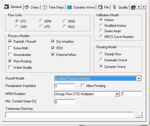
The runoff option is selected as shown in Figure 2 and the Storm parameters are entered as shown in Figure’s 3 and 4

Figure 2 Modified Rational Method is the last method in the Pull Down Menu in the Runoff Model Selection Dialog. As shown in

Figure 3 The parameters for the Modified Rational Method (Runoff Coefficient, Time of Concentration and Design Storm Tc Multiplier) can be added or edited in the Attribute Browser (AB) of InfoSWMM and H2Omap SWWMM. They can also be entered using the DB Tables as shown in

Figure 4 The parameters for the Modified Rational Method (Runoff Coefficient, Time of Concentration and Design Storm Tc Multiplier) can be added or edited in the Subcatchment DB Tables of InfoSWMM and H2Omap SWWMM.

The storm parameters of the MRM are shown in Figure 6 and Figure 7

Figure 5 The Modified Rational Method has a total storm depth and either a total storm duration or a time of concentration (tc) multiplier.

Figure 6 The duration of the Modified Rational Method (MRM) is either entered as absolute hours or a time of concentration (tc) multiplier

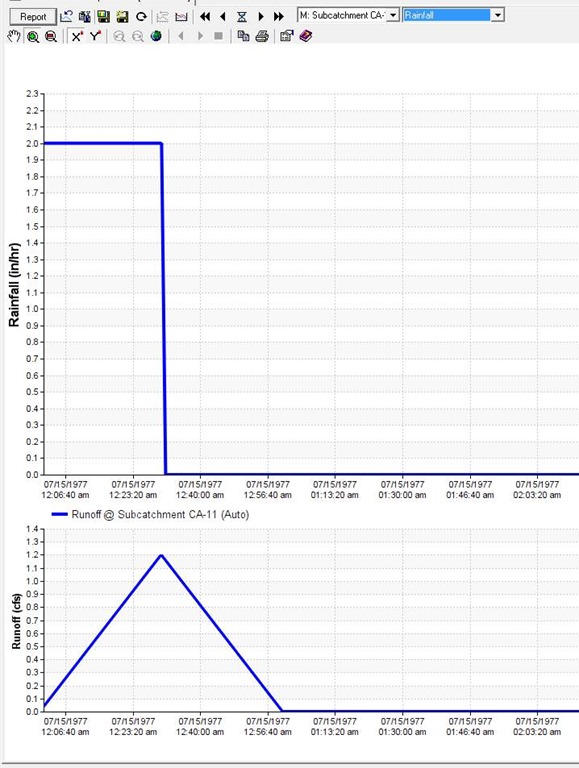
The output of the MRM Runoff Option as shown in Figure’s 7, 8 and 9

Figure 7 The Output Manager Subcatchment Summary Table shows the peak flow, the total runoff, the time of concentration and the Simulated Runoff Coefficient.

Figure 8 The Runoff Graph can be triangular based on a constant rainfall shape if the duration is set equal to zero.

Figure 9 The Runoff Graph can be trapezoidal based on a constant rainfall shape if the duration is non zero.

Figure 2 Modified Rational Method is the last method in the Pull Down Menu in the Runoff Model Selection Dialog.

Figure 3 The parameters for the Modified Rational Method (Runoff Coefficient, Time of Concentration and Design Storm Tc Multiplier) can be added or edited in the Attribute Browser (AB) of InfoSWMM and H2Omap SWWMM.

Figure 4 The parameters for the Modified Rational Method (Runoff Coefficient, Time of Concentration and Design Storm Tc Multiplier) can be added or edited in the Subcatchment DB Tables of InfoSWMM and H2Omap SWWMM.

Figure 5 The Modified Rational Method has a total storm depth and either a total storm duration or a time of concentration (Tc) multiplier.

Figure 6 The duration of the Modified Rational Method (MRM) is either entered as absolute hours or a time of concentration (Tc) multiplier

Figure 7 The Output Manager Subcatchment Summary Table shows the peak flow, the total runoff, the time of concentration and the Simulated Runoff Coefficient.

Figure 8 The Runoff Graph can be triangular based on a constant rainfall shape if the duration is set equal to zero.

Figure 9 The Runoff Graph can be trapezoidal based on a constant rainfall shape if the duration is non zero.