Tributary Area to a Node in SWMM 5 or InfoSWMM

Note:  Tributary Area to a Node in SWMM 5 or InfoSWMM

Here are the steps you neeed to take to calculate the tributary area of a node in InfoSWMM:

Step 1:  Use the DB Editor to get the total area in your model using the Data Statistics Tool.

Step 2:  Use the Process options in InfoSWMM to ONLY simulate surface runoff and flow routing.

Step 3. Copy the Node name and Total Inflow Volume from the Juntion Summary Output Table to Excel

Step 4:  Find the Total Wet Weather Flow during the simulation from the Wet Weather Inflow Row in the Flow Continuity Table.

Dry Weather Inflow   0.000  0.000

Wet Weather Inflow  0.782   0.255

Step 5. Make a new column in Excel to calculate the tributary area.

The Tributary Area of a Node = Total Inflow Volume / Total Wet Weather Flow * Total Subcatchment Area from Step 1.

You will now have the tributary area for each node.  You can verify this number = the total tributary area at the outfalls should equal the Total Subcatchment Areafrom Step 1.

		Maximum	Maximum
		Lateral	Total	Time	of	Lateral	Total	Tributary
		Inflow	Inflow	Occurrence	Volume	Inflow	Inflow	Area
Node	Type	CFS	CFS	days	hr:min	10^6 gal	10^6 gal	acres
P001	JUNCTION	5.54	10.86	0	2:27	0.1	0.255	14.74
P005	JUNCTION	2.14	7.42	0	2:26	0.039	0.155	8.96
P009	JUNCTION	5.78	5.78	0	2:25	0.106	0.106	6.13
P011	JUNCTION	0.7	0.7	0	2:34	0.01	0.01	0.58
OUTLET	OUTFALL	0	10.84	0	2:28	0	0.255	14.74

How to Set Up an InfoSWMM 2D Simulation Polygon and Mesh

Subject: How to Set Up an InfoSWMM 2D Simulation Polygon and Mesh

Step 1: Create the 2D Database

Step 2: Verify the Creation of the 2D Database

Step 3: Create the background Simulation Polygon for the 2D simulation

Step 4: Create the Mesh on the 2D Simulation Polygon

Step 5: Run the combination 1D and 2D network

Step 6: Simulating the network uses up to the number of cores on your computer for the 2D flow.

Step 7: 2D plot of the flooded mesh points.

Drainage Wells or a Vertical Exfiltration Trench in InfoSWMM

Subject:  Drainage Wells or a Vertical Exfiltration Trench in InfoSWMM

Note, this is just one way to model an Exfiltration Trench.  The source for the image below is Rice Creek Watershed. 

You can make a storage node to simulate the trench with the following characteristics:

·         Functional or Shape Curve to describe the shape of the trench,

·         Infiltration parameters to simulate the infiltration flow out of the bottom or sides of the trench,

Step 1:  Define the shape and geometrical characteristics of the Infiltration Trench

Step 2: Define the soil infiltration characteristics of the trench

Step 3:  Run the simulation.  The Storage Volume Summary tells you the volume infiltrated and the average outflow.

Step 4:  Output Manager will also show the infiltration  outflow, the depth and the volume of the infiltration/storage node.

Step 4:    Infiltration losses out the side and bottom of the orifice.

How to make Multiple Storm Events in InfoSWMM and How to Use them in the Scenario Manager

Subject:  How to make Multiple Storm Events in InfoSWMM and How to Use them in the Scenario Manager

Step 1.  Make a new Time Series to hold the data points for your new Rainfall Time Series in the Operation Tab of the Attribute Browser.

 

Step 2.  Populate the Rainfall Distribution with a SCS Type II Hyetograph with a 1 inch rainfall total

 

Step 3.  Now Clone the created Rainfall Distribution and make 10, 25, 50 and 100 year storm events each with 1 inches of rainfall in a cumulative distribution.

 

Step 4.  Now use the Block Edit command and convert each of the newly created hyetographs to 4, 7, 10, 15 and 20 inch cumulative rainfall totals from the original 1 inch rainfall total (for example).

Step 5.  Now create a Raingage for each of the newly created hyetograph time series using the DB Editor under the Raingage Table in Hydrologic Data

Step 6.  Link the Time Series to the new Raingages and define the type (cumulative), units (inches) and hyetograph interval (15 minutes)

Step 7. Make 4 New Scenarios for the different return period hyetographs,  the Base Scenario will use the 5 year or 4 inch SCS II rainfall.

Step 8. Use the DataSet Manager and make 4 new Subcatchment DB Tables in which each Subcatchment Set uses a different return period hyetograph.

Step 9. Run the Batch Simulator for all 5 scenarios including the Base Scenario.

Step 10.  You can  use the Output Report Manager to see the Rainfall for all of the Batch Runs to check if the proper rainfall was used for each Scenario Simulation.

Weirs in InfoSWMM and SWMM5

Weirs in InfoSWMM and SWMM5

Subject: Weirs in InfoSWMM

 Figure 1 shows the relationship between the weir input data and the upstream and  downstream nodes.

·         Height,

·         Crest and

·         Node Invert Elevation

 There are four types of weirs and if the weir becomes submerged downstream the Villemonte weir submergence correction is applied (Figure 2).  You can have flow reversal across the weir unless you use a Flap Gate for the weir (Figure 3). 

Figure 1:  Definition of Weir Terms

Figure 2: Villemonte Weir Submergence Correction

Figure 3:  Flow Reversal in a Weir

A Basic InfoSewer Wet Well, Pump and Force Main System

Note:  A Basic InfoSewer Wet Well,  Pump and  Force Main System

How is the St Venant Equation Solved for in the Dynamic Wave Solution of SWMM 5?

Subject:   How is the St Venant Equation Solved for in the Dynamic Wave Solution of SWMM 5?

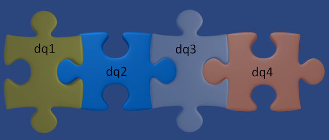
An explanation of the four St. Venant Terms in SWMM 5 and how they change for Gravity Mains and Force Mains. The HGL is the water surface elevation in the upstream and downstream nodes of the link. The HGL for a full link goes from the pipe crown elevation up to the rim elevation of the node + the surcharge depth of the node.  The four terms are:

dq2 = Time Step * Awtd * (Head Downstream – Head Upstream) / Link Length or

dq2 = Time Step * Awtd * (HGL) / Link Length

Qnew = (Qold – dq2 + dq3 + dq4) / ( 1 + dq1)

when the force main is full dq3 and dq4 are zero and

Qnew = (Qold – dq2) / ( 1 + dq1)

The dq4 term in dynamic.c uses the area upstream (a1) and area downstream (a2), the midpoint velocity, the sigma factor (a function of the link Froude number), the link length and the time step or

dq4 = Time Step * Velocity * Velocity * (a2 – a1) / Link Length * Sigma

the dq3 term in dynamic.c uses the current midpoint area (a function of the midpoint depth), the sigma factor and the midpoint velocity

dq3 = 2 * Velocity * ( Amid(current iteration) – Amid (last time step) * Sigma

dq1 = Time Step * RoughFactor / Rwtd^1.333 * |Velocity|

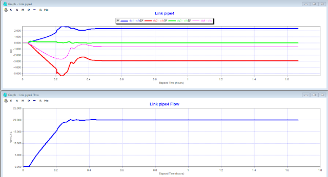
The weighted area (Awtd) is used in the dq2 term of the St. Venant equation:

dq2 = Time Step * Awtd * (Head Downstream – Head Upstream) / Link Length

The four terms change at each iteration and time step to determine the new flow (Figure 1) based on the two equations:

Denom = 1 + dq1 + dq5

Q = [Qold – dq2 + dq3 + dq4] / Denom

If you look at a table of the values you will see that the terms add up to zero when the flow is constant and to delta Q or the change in Q when the flow is NOT constant (Figure 2).

Figure 1.  The four terms define the new flow at each iteration in the dynamic wave solution of SWMM5

  

Figure 2.   The magnitude of the four terms determine the flow at the new iteration and ultimately the new Time Step.  If the flow is constant then the value of the term is constant.