Showing posts with label #SWMM5. Show all posts

Monday, July 10, 2017

The relationship between the current link mid point velocity and the time step in a link of #SWMM5

SWMM5 uses the Courant–Friedrichs–Lewy (CFL) condition to compute the variable time step used during each time step of a simulation.   In general, the shortest link length with the highest velocity and depth will dominate the time step computations.   The CFL time step is the link length over the current velocity plus the current wave celerity.  If you plot the velocity and computed time step over time the time step will decrease as the velocity increases (Figure 1).  Figure 1 also shows why a hot start file is important in SWMM5.  If you start out with a dry network the SWMM5 engine will not be able to have a good estimate of the needed CFL time step.  The depth and velocity will be zero.

Figure 1 - The relationship between the current link mid point velocity and the time step in a link of SWMM5.

Sunday, June 25, 2017

World Class Software Documentation for SWMM5 from Lew Rossman and Wayne Huber (Hydrology)

I posted this on the SWMM Group on LinkedIn
I have noticed based on email questions and postings to the SWMM LIst Sever (a great resource hosted by CHI, Inc.) that many SWMM 5 users do not know about the really outstanding documentation on SWMM 5 posted on the EPA Website https://www.epa.gov/water-research/storm-water-management-model-swmm It consists of two now and in the near future three volumes on Hydrology, Water Quality, LID’s and SuDs and Hydraulics. The documentation is fantastically complete with detailed background on the theory, process parameters and completely worked out examples for all of the processes in SWMM5. It is truly an outstanding aid to modelers and modellers worldwide. It would benefit you to read them (if you have not already downloaded the PDF files). Thanks for reading this post

Saturday, March 4, 2017

For Thesis Students: Visual INSTRUCTIONS FOR COMPILING SWMM5.DLL USING MICROSOFT VISUAL C++ 2010/2012

For Thesis Students:  Visual INSTRUCTIONS FOR COMPILING SWMM5.DLL USING MICROSOFT VISUAL C++ 2010/2012
=========================
The following is based on the readme.txt for compiling that EPA distributes with the SWMM5 install

1. Open the file swmm5.c in a text editor and make sure that the
   compiler directives at the top of the file read as follows:
       //#define CLE
       //#define SOL
       #define DLL   or the DLL will be created

2. Create a sub-directory named VC2010_DLL under the directory where
   the SWMM 5 Engine source code files are stored and copy SWMM5.DEF
   and VC2010-DLL.VCPROJ to it.

3. Launch Visual C++ 2010 and use the File / Open command to open
   the VC2010-DLL.VCPROJ file.

4. Issue the Build >> Configuration Manager command and select the
   Release configuration.

5. Issue the Build VC2010-DLL command to build SWMM5.DLL
   (which will appear in the Release subdirectory underneath the
   VC2010-DLL directory).

NOTE: The VC-2010 project file includes Open MP support which is
      only available with the Professional and higher versions of
      the compiler.

A SmartArt view of the process


How it looks in the Windows directory

C:\SWMMandSoftware\VisualStudioSWMM5\swmm51010_engine\VC2010_DLL

Arbitrary Windows directory name with a Subfolder of the SWMM 5 engine followed by a Subfolder called VC2010_DLL with files SWMM5.DEF
   and VC2010-DLL.VCPROJ


How it looks in Visual Studio 2012

And here is how it compiles right away
1>  Generating Code...
1>  Compiling...
1>  shape.c
1>  snow.c
1>  stats.c
1>  statsrpt.c
1>  subcatch.c
1>  surfqual.c
1>  swmm5.c
1>  table.c
1>  toposort.c
1>  transect.c
1>  treatmnt.c
1>  xsect.c
1>  Generating Code...
1>     Creating library C:\SWMMandSoftware\VisualStudioSWMM5\swmm51010_engine\VC2010_DLL\Debug\VC2010-DLL.lib and object C:\SWMMandSoftware\VisualStudioSWMM5\swmm51010_engine\VC2010_DLL\Debug\VC2010-DLL.exp
1>  VC2010-DLL.vcxproj -> C:\SWMMandSoftware\VisualStudioSWMM5\swmm51010_engine\VC2010_DLL\Debug\VC2010-DLL.dll
========== Build: 1 succeeded, 0 failed, 0 up-to-date, 0 skipped ==========

If you want the Release version use Build/Release


Note on April 28, 2017 - I am including a link to a zip file of a working directory in VS 2012 and the directory C:\SWMMandSoftware\swmm51012_engine
You can download the entire directory (working using this link) http://blog.innovyze.com/wp-content/uploads/2016/09/swmm51012_engine.ziphttp://blog.innovyze.com/wp-content/uploads/2016/09/swmm51012_engine.zip

Sunday, October 23, 2016

How to Use Scatter Plots in the DB Output tables of #InfoSWMM for d/D and q/Q


Harness the power of visualization with scatter plots in the DB Output tables of #InfoSWMM—a dynamic feature that brings the extensive data from SWMM5 output tables to life. 🌟📊

In InfoSWMM, you're not just reading numbers; you're witnessing the maximum link values dance across the Conduit Summary Table. With a simple right-click, a world of statistical analysis unfolds before you, offering plots, frequency graphs, histograms, and the coveted scatter graphs for any selected column. 🖱️💡

Dive Into the Data: Engage in a visual dialogue with your model by selecting two columns and crafting a scatter plot that tells a story. A plot of particular interest? The relationship between d/D, the depth-to-diameter ratio (capacity) of the pipe, and q/Qfull, the flow rate to full capacity flow rate. 📈🔍

Why Does It Matter? Qfull is calculated based on the full pipe depth, area, and hydraulic radius, all derived from the bed slope. Given that InfoSWMM, SWMM5 employ the robust St. Venant equations, you might observe q/Qfull ratios exceeding 1, even when d/D is below 1—a testament to the detailed physics captured by the models. 🌊🔢

Reference Material: For those thirsty for more knowledge, a treasure trove of St. Venant solutions within SWMM5 awaits in our comprehensive blogs. Each post serves as a beacon, guiding you through the intricacies of hydraulic modeling. 📚✨

Embrace these tools to transform data points into a narrative, charting the course of your wastewater management journey with precision and clarity. 🛠️🌐🚀


Figure 1 - How to Use Scatter Plots in the DB Output tables of #InfoSWMM for d/D and q/Q

Update for [USEPA/SWMM-EPANET_User_Interface] MTP 3

Just a note about the great work being done on the new EPANET and SWMM 5 QGIS interface.
This is the third Minimum Testable Product, released for testing of specific functionality.
This is not a fully functional product and is not suitable for production use.

You are receiving this because you are subscribed to this thread.
View it on GitHub 

Sunday, October 16, 2016

More St Venant Equations in #SWMM5

This blog shows the relationship between the terms dq1, dq2, dq3 and dq4 in the SWMM5 code and the St. Venant Partial Differential Equations.

dq2 = Time Step * Area wtd * (Head Downstream – Head Upstream) / Link Length or

dq2 = Time Step * Area wtd * (HGL) / Link Length Qnew = (Qold – dq2 + dq3 + dq4) / ( 1 + dq1) when the force main is full dq3 and dq4 are zero and

Qnew = (Qold – dq2) / ( 1 + dq1) The dq4 term in dynamic.c uses the area upstream (a1) and area downstream (a2), the midpoint velocity, the sigma factor (a function of the link Froude number), the link length and the time step or

dq4 = Time Step * Velocity * Velocity * (a2 – a1) / Link Length * Sigma the dq3 term in dynamic.c uses the current midpoint area (a function of the midpoint depth), the sigma factor and the midpoint velocity

dq3 = 2 * Velocity * ( Amid(current iteration) – Amid (last time step) * Sigma

dq1 = Time Step * RoughFactor / Rwtd^1.333 * |Velocity| The weighted area (Awtd) is used in the dq2 term of the St. Venant equation:

dq2 = Time Step * Awtd * (Head Downstream – Head Upstream) / Link Length


In this blog we show how the St Venant terms are used in SWMM5 as equations, table, graphs and units. We use a QA/QC version of SWMM 5 that lists many more link, node, system and Subcatchment variables than the default SWMM 5 GUI and engine. This also applies to #InfoSWMM and any software the uses the #SWMM5 engine.  
SWMM5 is using is the most advanced equations as it takes into consideration the full dynamic (St. Venant) equations and not the more simplified kinematic wave / manning equations. The manning equation only considers the uniform flow conditions which represents a situation where the gravitational force on a column of water (due to the channel slope) balances out the frictional force. The full dynamic equations contains additional factors that affect the movement of water in a conduit or channel. These include the pressure force due to variation of depth along the length of the channel and the inertial (or convective acceleration) effect due to variation of flow area along the channel length. Because of these additional terms the flow/head relation you have in uniform flow conditions can be completely different according to the configuration of his network.

Saturday, October 15, 2016

#SWMM5 1-D St Venant Equation Terms

Overview

In this blog we show how the St Venant terms are used in SWMM5 as equations, table, graphs and units. We use a QA/QC version of SWMM 5 that lists many more link, node, system and Subcatchment variables than the default SWMM 5 GUI and engine. This also applies to #InfoSWMM and any software the uses the #SWMM5 engine.
SWMM5 is using is the most advanced equations as it takes into consideration the full dynamic (St. Venant) equations and not the more simplified kinematic wave / manning equations. The manning equation only considers the uniform flow conditions which represents a situation where the gravitational force on a column of water (due to the channel slope) balances out the frictional force. The full dynamic equations contains additional factors that affect the movement of water in a conduit or channel. These include the pressure force due to variation of depth along the length of the channel and the inertial (or convective acceleration) effect due to variation of flow area along the channel length. Because of these additional terms the flow/head relation you have in uniform flow conditions can be completely different according to the configuration of his network.

How are the St Venant Terms used in SWMM5?

Figure 1 shows the terms and Figure 2  and Figure 3 shows the terms in a SWMM5 table and SWMM5 graph. 

dq2 = Time Step * Area wtd * (Head Downstream – Head Upstream) / Link Length or

dq2 = Time Step * Area wtd * (HGL) / Link Length Qnew = (Qold – dq2 + dq3 + dq4) / ( 1 + dq1) when the force main is full dq3 and dq4 are zero and

Qnew = (Qold – dq2) / ( 1 + dq1) The dq4 term in dynamic.c uses the area upstream (a1) and area downstream (a2), the midpoint velocity, the sigma factor (a function of the link Froude number), the link length and the time step or

dq4 = Time Step * Velocity * Velocity * (a2 – a1) / Link Length * Sigma the dq3 term in dynamic.c uses the current midpoint area (a function of the midpoint depth), the sigma factor and the midpoint velocity

dq3 = 2 * Velocity * ( Amid(current iteration) – Amid (last time step) * Sigma

dq1 = Time Step * RoughFactor / Rwtd^1.333 * |Velocity| The weighted area (Awtd) is used in the dq2 term of the St. Venant equation:

dq2 = Time Step * Awtd * (Head Downstream – Head Upstream) / Link Length

You can also see the QA/QC report for SWMM 5 https://www.epa.gov/water-research/storm-water-management-model-swmm#downloads

How are the St Venant Units used in #SWMM5?

The new flow (Q) calculated at during each iteration of time step as

(1) Q for the new iteration = (Q at the Old Time Step – DQ2 + DQ3 + DQ4 ) / ( 1.0 + DQ1 + DQ5)

In which DQ2, DQ3 and DQ4 all have units of flow (note internally SWMM 5 has units of CFS and the flows are converted to the user units in the output file, graphs and tables of SWMM 5).

The equations and units for DQ2, DQ3 and DQ4 are:

(2) Units of DQ2 = DT * GRAVITY * aWtd * ( H2 – H1) / Length = second * feet/second^2 * feet^2 * feet / feet = feet^3/second = CFS

(3) Units of DQ3 = 2 * Velocity * ( aMid – aOld) * Sigma = feet/second * feet^2 = feet^3/second = CFS

(4) Units of DQ4 = DT * Velocity * Velocity * ( aMid – aOld) * Sigma / Length = second * feet/second * feet/second * feet^2 / feet = feet^3/second = CFS

The equations and units for DQ1 and DQ5 are:

(5) Units of DQ1 = DT * GRAVITY * (n/PHI)^2 * Velocity / Hydraulic Radius^1.333 = second * feet/second^2 * second^2 * feet^1/3 * feet/second / feet^1.33 = Dimensionless

(6) Units of DQ5 = K * Q / Area / 2 / Length * DT = feet^3/second * 1/feet^2 * 1/feet * second = Dimensionless
Figure 1.  St Venant Terms in Table and Graphs for #SWMM5 for dq1, dq2, dq3, dq4, dq5, dq6

Figure 2.  St Venant Equation in SWMM5

Sunday, May 1, 2016

Why is a Hot Start File important in SWMM 5 and InfoSWMM

A Hot Start File in InfoSWMM  or SWMM 5 is important as it provides initial   depths, initial flows and  initial settings for the hydrology and hydraulics features of the SWMM 5 engine.    You  have three options:
  1. Save a hot Start File at the  end of the  simulation,
  2. Use a hot Start File  at the beginning of  the simulation,
  3. Create a hot start file  from  the a  time during  the  Map Display
If you change any of the network  types or add new links and nodes then  the Hot Start file needes to be recreated.  InfoSWMM use the Tab File in  the Run Manager to name the Hot Start File (Figure 1).   Each and  every Scenario in InfoSWMM  can  use or Save a different scenario with different starting  and ending  times  (Figure 2).  If you USE  a Hot  Start  File then:
  1. The  new  simulation  starts at the end  of  the  old  simulation
  2. You can  run a Quasi Steady State Simulation and use a very short simulation time of minutes if you use a Hot Start File
  3. Figure 3  shows  the effect of Using a Hot Start File
hs4
Figure 1. File Tab for Saving or Using a  Hot Start file in InfoSWMM  or  H2OMap SWMM.   There  is  a similar dialog in  SWMM5.
hs3
Figure 2.  Each Scenario in  InfoSWMM  and  H2OMap  SWMM can have a   different set of report  and simulation options.


HS100
Figure 3.   The Saved Time Series for the  Outfall (Blue) and  Use (Green)  Outfall  Time Series.

Tuesday, February 23, 2016

Innovyze Further Expands RDII Analyst Functionality, Setting New Standard for Sanitary and Combined Sewer System Model Calibration

Innovyze Further Expands RDII Analyst Functionality, Setting New Standard for Sanitary and Combined Sewer System Model Calibration

New Features Allow Unprecedented Analysis and Comparison of Rainfall-Derived Inflow and Infiltration Data, Parameters for Complex Sewers

Broomfield, Colorado, USA, February 23, 2016

Innovyze, a leading global innovator of business analytics software and technologies for smart wet infrastructure, today announced the newest release of its RDII Analyst (Rainfall-Derived Inflow and Infiltration) for InfoSWMM and H2OMAP SWMM. The new version delivers expanded functionality, incorporating many advanced Genetic Algorithm (GA) optimization features. It increases its unmatched productivity by openly inviting the users to further adjust the dry weather flow (DWF) and RTK parameters (with initial and maximum monthly storages for continuous simulation) to achieve a better fit and ultimately a better model based on their experiences. The release confirms Innovyze’s commitment to giving the world the most complete toolset for modeling current sanitary and combined sewer collection systems.

Excessive wet weather flow from rainfall-derived manhole and pipe defect inflow and infiltration is a major source of sanitary and combined sewer overflows. Controlling these overflows is vital in reducing risks to public health and protecting the environment from water pollution. Computer modeling plays an important role in determining sound and economical remedial solutions that reduce RDII; improve system integrity, reliability and performance; and avoid overflows.

The processes for converting rainfall to RDII flow in sanitary sewer systems are very complicated. In addition to rainfall and antecedent moisture conditions, factors controlling RDII responses include depth to groundwater, depth to bedrock, land slope, number and size of sewer system defects, type of storm drainage system, soil characteristics, and type of sewer backfill. Given this degree of complexity, flow-monitoring data must be combined with mathematical modeling and analytics to provide accurate results. The wastewater flow monitoring data obtained by sewer collection systems consists of dry-weather flow components, ground water flow and twelve (12) RDII flow components. A crucial step in successfully modeling sewer collection systems is the ability to decompose flow-monitoring data into RDII flow, ground water flow and dry weather flow and its flow pattern.

Significantly superior to the EPA Sanitary Sewer Overflow Analysis and Planning (SSOAP) program and powered by advanced GA optimization and comprehensive data analytics and scenario management, RDII Analyst provides the ability to quickly and reliably perform these types of advanced flow decomposition data monitoring. It has been updated with tabular comparisons between the observed and calibrated RDII data for each event, including R value, peak flow, hydrograph volume and depth. This allows the user to better evaluate simulated and monitored data and judge how well it correlates on a per event basis. The user can also directly edit estimated DWF mean values to apply site specific knowledge to the RDII Analyst DWF extraction algorithm. These altered DWF values can then be used to estimate the wet weather flow component of the monitored flow, using a combination of the DWF extraction algorithm and site-specific knowledge. The new version also allows direct edits to the twelve RTK and storage parameters plus manual curve fitting to apply site specific knowledge to the genetic algorithm parameter estimation. Manual curve fitting is valuable in timing differences between monitored and calibrated wet weather flow components and employing previous experience in estimating RTK parameters.

“Innovyze continues to listen to our customers, invest very heavily in R&D, and deliver the advanced tools they need to effectively support their wastewater and urban drainage modeling and management challenges,” said Paul F. Boulos, Ph.D., BCEEM, Hon.D.WRE, Dist.D.NE, Dist.M.ASCE, NAE, President, COO and Chief Technical Officer of Innovyze. “We are very excited that our vast worldwide customer base will now be able to use the powerful new features in RDII Analyst to enhance their modeling experiences, wrap better projects faster, and strengthen our communities’ sewer systems.”

Pricing and Availability
Upgrade to RDII Analyst is now available worldwide by subscription to the Executive program. Subscription members can immediately download the new version free of charge directly from www.innovyze.com. The Innovyze Subscription Program is a friendly customer support and software maintenance program that ensures the longevity and usefulness of Innovyze products. It gives subscribers instant access to new functionality as it is developed, along with automatic software updates and upgrades. For the latest information on the Innovyze Subscription Program, visit www.innovyze.com or contact your local Innovyze Channel Partner.
About InnovyzeInnovyze is a leading global provider of wet infrastructure business analytics software solutions designed to meet the technological needs of water/wastewater utilities, government agencies, and engineering organizations worldwide. Its clients include the majority of the largest UK, Australasian, East Asian and North American cities, foremost utilities on all five continents, and ENR top-rated design firms. With unparalleled expertise and offices in North America, Europe and Asia Pacific, the Innovyze connected portfolio of best-in-class product lines empowers thousands of engineers to competitively plan, manage, design, protect, operate and sustain highly efficient and reliable infrastructure systems, and provides an enduring platform for customer success. For more information, call Innovyze at +1 626-568-6868, or visit www.innovyze.com.
Innovyze Contact:Rajan RayDirector of Marketing and Client Service Manager
Rajan.Ray@innovyze.com
+1 626-568-6868
- See more at: http://www.innovyze.com/news/1664/#sthash.VMYZZnmf.dpuf

Saturday, February 6, 2016

Innovyze RDII Analyst for the Analysis and Calibration of RDII, DWF, DWF Patterns and GWI in Sewer Collection Systems

One of the most powerful InfoSWMM, InfoSWMM SA and H2OMAP SWMM Application Tools from Innovyze is RDII Analyst.  RDII Analyst will separate out the Groundwater base flow, Dry Weather Flow (DWF), DWF Patterns, estimate the Wet Weather flow component or RDII  Rainfall -Derived Infiltration Inflow (I&I) and use a Genetic Algorithm to find  the best fit 12 RTK parameters for RDII modeling.  This powerful tool can  be used for RTK flow in InfoSWMM, H2OMAP SWMM, InfoSewer, SWMM 5 and InfoWorks ICM.  Figure 1 shows one of the  end results of RDII Analyst – a correlation plot of Observed versus Calibrated RDII Volume for the simulated events.
RDII Analyst is a significant improvement over the EPA SSOAP program, performs QA/QC of rainfall and flow monitoring data and decomposes the flow data into Dry-Weather Flow (DWF) and Wet-Weather Flow (RDII) components using criteria such as rainfall threshold. The DWF component is further analyzed to construct a DWF pattern that can be used to simulate the collection system using InfoSWMM. The DWF pattern is then assigned to the source nodes that contribute DWF to the meter location in proportion to sewershed areas or based on other criteria. The RDII component is then analyzed to determine RDII events and to calibrate parameters of the RTK synthetic unit hydrograph so that the RDII flow simulated by the RTK method closely matches the RDII flow obtained by the decomposition process. The RTK unit hydrograph parameters are calibrated with genetic algorithm optimization. The calibrated RTK parameters and the DWF patterns are then passed to InfoSWMM to carry out detailed dynamic flow routing through the sewer system and evaluate system response to support the development of an optimal capital improvement program. You can read the World Environmental and Water Resources Congress paper by Misgana and Boulos (2008) with a complete description and validation of the RDII Analyst workflow process for both RDII Analyst and for the InfoSWMM Calibrator Add-On in the InfoSWMM Suite (Boulos, 2005)
RDII00002
Figure 1. Correlation plot of Observed versus Calibrated RDII Volume for the simulated events.
The steps in using RDII Analyst are both simple and powerful, the main steps are:
  • Import flow monitoring data and rainfall data into RDII Analyst
  • Perform QA/QC for the flow data and the rainfall data
  • Determine dry day flows and create hourly DWF pattern for weekend and weekdays
  • Determine the groundwater flow component of the dry days flows
  • Determine RDII flow time series
  • Identify RDII events, and perform linear regression analysis on the RDII depth and rainfall depth calculated for each RDII event
  • Run Genetic Algorithms based calibration of the RTK hydrograph parameters and review calibration results
  • Export the DWF patterns, the GWF time series and the calibrated RTK parameters to InfoSWMM
In this overview of the steps in the remainder of the blog post, you’ll learn how the RDII Analyst tool works in general and what terminology is used to describe each step. This is recommended reading for anyone who is new to RDII Analyst.  If you are experienced in RDII decomposition, you can probably just skim it when needed.

Step 1.  Define the Flow and Rainfall Data

The flow and rainfall data are imported by each monitored Node location.  The flow and  rainfall format are defined along with the monitored data time intervals.  The rainfall and flow do not have to be at the same interval or cover exactly the same time period. The Flow Data Tab displays the flow data that has been read from the flow data file. The display consists of the data area showing Date Time and Value field that is read from the data file. The Rainfall Data Tab displays the flow data that has been read from the rainfall data file. The display consists of the data area showing Date Time and Value field that is read from the data file.
Figure 2. Imported Flow Data in RDII Analyst
Figure 3. Imported Rainfall Data in RDII Analyst

Step 2.  DWF Extraction

The DWF Mean and Patterns are extracted from the Flow Time Series and the residual is used as the basis of the RTK parameter estimation. The dry day flows identified for weekdays and the weekend are further analyzed to determine hourly DWF patterns that can be used to model DWF in InfoSWMM . The DWF pattern presents average hourly DWF values across all dry days for both weekdays and weekend. The DWF pattern is given both graphically and in report form as shown below. The DWF patterns can be exported to InfoSWMM and are assigned to nodes that contribute flow to the meter location proportional to sewershed area or equally among all nodes.
Once determined, the dry days flows are presented both in report form and in graph form for weekend and for weekdays as shown below. The graph shows average daily flow for each dry day, and upper bound and the lower bounds. The upper bound refers to mean flow of all dry day flows plus standard deviation multiplier *standard deviation of dry day flows. The lower bound refers to mean flow of all dry day flows minus standard deviation multiplier *standard deviation of dry day flows. The bounds help the user visually identify outliers and, if necessary, discard those days from further consideration.
Figure 4. Define the Methods used in the DWF Extraction.
Figure 5. Mean and QA/QC Graph for the DWF Extraction.
Figure 6. DWF Pattern found by RDII Analyst
Figure 7. Estimated Weekly GroundWater Flow.

Step 3.  Ground Water Base Flow Extraction

The DWF Mean and Patterns are extracted from the Flow Time Series and the residual is used as the basis of the RTK parameter estimation.  As part of the DWF Extraction, the GW flow can be estimated and later exported to InfoSWMM and a Time Series (Figure 7). The groundwater flow time series can be exported to InfoSWMM as external inflow and can be assigned to nodes that contribute flow to the meter location proportional to sewershed area or equally among all nodes.

Step 4.  Export DWF Pattern and DWF Means to the Domain in InfoSWMM

Assign DWF Pattern: This tool assigns the hourly DWF patterns developed for weekdays and weekends to InfoSWMM nodes that contribute flow to the monitoring site. The DWF pattern is allocated to the contributing nodes either proportional to sewershed area of each contributing node, or simply equally among all contributing nodes. The user must assign an ID to be used as the weekday and weekend pattern name. The assignment could be limited to nodes in a domain by checking the Assign to Domain Nodes option.
Figure 8. Export Dialog to export the DWF means and DWF patterns to the Node DWF DB Table or the Patterns DB Table in InfoSWMM.

Step 5.  Create the RDIII or Wet Weather Time Series

RDII flow is the difference between the corrected monitoring flow data, and the sum of average hourly DWF pattern and the groundwater flow time series. Once the hourly DWF pattern and the groundwater flow components are identified, the sum of the two components would be subtracted from the corrected flow data to determine the RDII flow component.
Figure 9. The estimated WWF or RDII time series after extaction fo the mean DWF and DWF Pattern.
Figure 9. The estimated WWF or RDII time series after extaction fo the mean DWF and DWF Pattern.

Step 6.  Calibrate the 12 RDII Parameters

One of the objectives of decomposing flow monitoring data into dry weather flow and wet weather flow components is to improve the accuracy of modeling the wet-weather flow component. In H2OMAP SWMM, RDII flow is modeled using the RTK method as previously described. The RTK method requires definition of up to 12 parameters. Proper choice of these parameters is crucial for accurate modeling of the RDII flow. Traditionally, RDII UH parameters are assigned using a tedious and inexact trial-and-error process in which the parameters are manually adjusted in an iterative fashion to closely match wet-weather flow data with the RDII flow generated by the simulation model using the assumed RTK parameters. Since there are a vast number of possible combinations of RTK values, evaluating all options this way may not be manageable, and even knowledgeable modelers often fail to obtain good results. RDII Analyst uses Genetic Algorithms (GA) optimization to automatically determine the UH parameters that best match the RDII time series generated by the RDII Analyst with the RDII flow estimated using H2OMAP SWMM.
The RDII calibration tool is launched using Analysis -> Calibrate RDII Parameters or using from tools. Minimum and maximum value for each parameter should be defined using the RTK Parameters Range dialog editor.
The calibration tool systematically searches for the best set of parameters that matches the RDII flow simulated by H2OMAP SWMM with RDII time series determined by the decomposition process. The parameter values would be searched within the minimum and the maximum ranges assigned by the user on dialog editor shown above. The model would adjust the nominal parameter values assigned by the user on H2OMAP SWMM RDII hydrograph dialog editor (see below) by a randomly selected multiplier within the range assigned for the parameter and chooses the optimal set of adjustments. The Tributary Area may be taken from the sewershed area defined in H2OMAP SWMM’s Hydrograph page, or the user can directly specify area of the tributary sewersheds. In addition, the user has the option to use sewershed area of the nodes defined in a domain. The Ensure that R1>R2>R3 option ensures that the RDII flow contributed by the first triangle (fast flow contribution) would be higher than contribution of the second triangle (intermediate flow), and contribution of the second triangle would be higher than that of the third triangle (slow flow).
Domain Node option is checked, sewershed area of the nodes included in the domain will be considered. Nodes in the domain will not contribute sewershed area. Once the parameters are assigned, hitting the OK button would initiate the calibration dialog box (see below).
Options: Some Genetic Algorithms (GAs) parameters may be defined using the options page initiated by clicking the Options button on the Calibrate RDII Parameters dialog box.
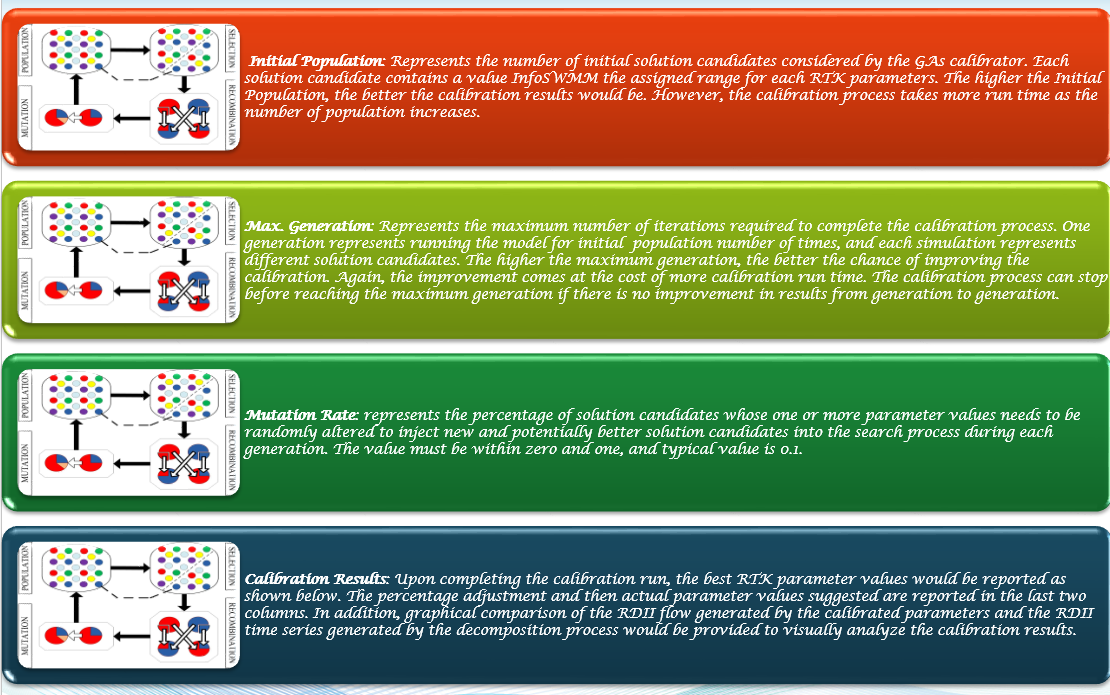
Initial Population: Represents the number of initial solution candidates considered by the GAs calibrator. Each solution candidate contains a value H2OMAP SWMM the assigned range for each RTK parameters. The higher the Initial Population, the better the calibration results would be. However, the calibration process takes more run time as the number of population increases.
Max. Generation: Represents the maximum number of iterations required to complete the calibration process. One generation represents running the model for initial population number of times, and each simulation represents different solution candidates. The higher the maximum generation, the better the chance of improving the calibration. Again, the improvement comes at the cost of more calibration run time. The calibration process can stop before reaching the maximum generation if there is no improvement in results from generation to generation.
Mutation Rate: represents the percentage of solution candidates whose one or more parameter values needs to be randomly altered to inject new and potentially better solution candidates into the search process during each generation. The value must be within zero and one, and typical value is 0.1.
Calibration Results: Upon completing the calibration run, the best RTK parameter values would be reported as shown below. The percentage adjustment and then actual parameter values suggested are reported in the last two columns. In addition, graphical comparison of the RDII flow generated by the calibrated parameters and the RDII time series generated by the decomposition process would be provided to visually analyze the calibration results
Figure 10. The 12 RTK parameters can be estimated with min and max constraints to find the best fit parameters.

Step 7.  Examine the Calibration Report

The number of trial runs made so far, the maximum number of trials to be made and the best fitness obtained from the trail runs made so far would be shown while the model is running. If there is no significant improvement in the fitness for some time (i.e., from generation to generation), then the calibration process would be stopped. Once the calibration run is completed, the RDII flow simulated by the optimal RTK parameters identified by the calibration process would be compared graphically with the RDII time series obtained from the decomposition process. In addition, the optimal RTK parameters identified by the model would also be presented in table form.
RDII Analyst can further analyze the RDII time series to identify RDII events. Breaking RDII time series into separate events can enable a better understanding of the RDII process and aid in process of calibrating the model. Event definition depends on the values assigned for the inputs given in the RDII EVENT IDENTIFICATION dialog box shown below.
Minimum Rainfall Volume: represents the minimum rainfall depth that needs to be collected from “continuous” rain to initiate an event. By continuous rain, it means that for two rainfall occurrences to be considered as one event the time interval between the successive rains should not exceed the interevent time threshold defined by the user.
Minimum RDII Flow: represents the minimum RDII flow that should be generated as the result of the rainfall collected over the duration to accept the occurrence as an event.
Minimum Length of the Event (hr): refers to the minimum length of time that the RDII flow should exceed the minimum RDII flow for the occurrence to be accepted as an event.
Interevent Time Threshold (hr): refers to the length of time needed to separate two successive events. If two rainfall occurrences are separated by duration shorter than the Interevent Time Threshold, then the two rainfall occurrences are considered as one event.
Length of Time for Rain to become RDII (hr): This input refers to average time span for a rainfall event to start contributing RDII to the collection system. Depending on this input, the RDII event identification algorithm tests if an RDII flow has occurred within the Length of Time for Rain to become RDII (hr) after a rainfall event.
Tributary Area: This input is used to compute RDII flow depth based on RDII flow volume determined for each event. RDII Analyst can use the sewershed area defined in InfoSWMM’s RTK Hydrograph page, or the user can directly specify area of the tributary sewersheds. In addition, the user has the option to use sewershed area of the nodes defined in a domain. If the Use Domain Node option is checked, sewershed area of the nodes included in the domain will be considered. Nodes in the domain will not contribute sewershed area.
Figure 11. A Calibration Graph of the Monitored and Predicted RDII Time Series.

Step 8. RDII Event Analysis Results

Linear Regression Results: A linear regression equation is developed between the RDII depth and rainfall depth identified for each event. Slope of the regression equation represents the fraction of rainfall depth that enters the sewer system in the form of RDII (i.e., a representative R for all events).
Figure 12. Correlation plot of Observed versus Calibrated RDII Volume for the simulated events.

Step 9.  Export the RDII RTK Parameters to InfoSWMM

This function assigns either the RTK parameters determined by the calibration tool or the RDII time series determined by decomposing the flow monitoring data to InfoSWMM nodes that contribute flow to the monitoring site. The RTK parameters could be exported to InfoSWMM and assigned to RDII hydrographs for each contributing node. The time series is assigned to the nodes as external inflow. The RDII time series is allocated to the contributing nodes either proportional to sewershed area of each contributing node, or simply equally among all contributing nodes. The user must provide a name for the Hydrograph and/or the Time Series. The assignment could be limited to nodes in a domain by checking the Assign to Domain Nodes option. Please note that if both the GWF time series and the RDII time series are exported into InfoSWMM , only the time series exported last would be available for use. InfoSWMM takes only one exported external inflow time series at a time.
Figure 13. The 12 RTK parameters can now be exported back to InfoSWMM and H2OMAP SWMM.
Figure 14. The 12 RTK parameters in the Operations tab of the InfoSWMM Attribute Browser.
Figure 15. GA options in RDII Analyst
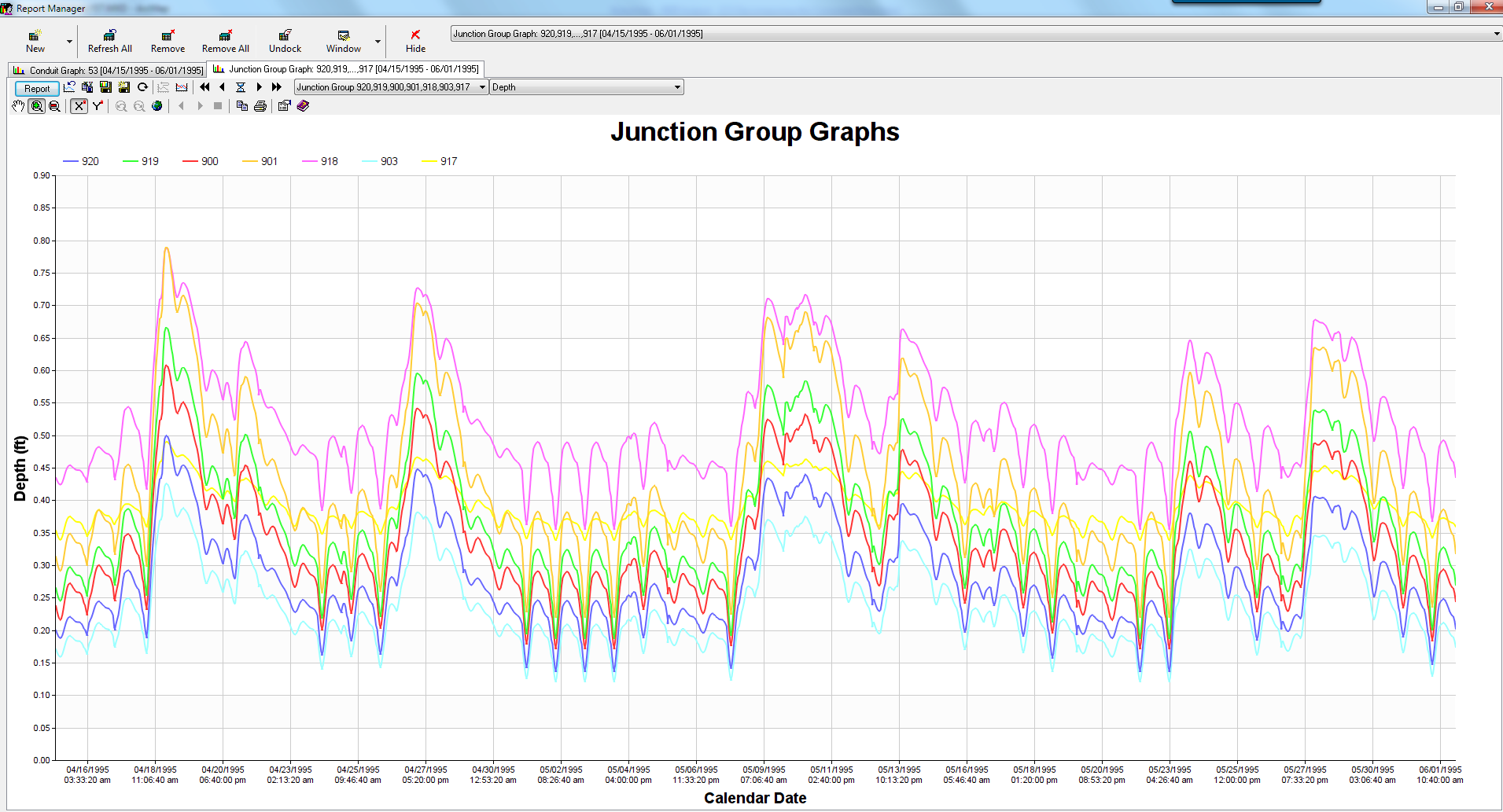
Figure 16. How the Exported DWF looks in InfoSWMM graphs of lateral flow at nodes

Saturday, January 16, 2016

A few connected tweets about #LID or #SuDS, #SWMM5, #INFOSWMM, #YOUTUBE and #INFOSEWER

A few connected tweets about #LID or #SuDS, #SWMM5, #INFOSWMM, #YOUTUBE and #INFOSEWER

via Low impact development a natural way to manage .
Embedded image permalink

2/ One of the Subscribed H&H Channels is for all Software on YouTube
Embedded image permalink

1/ The YouTube channel is getting close to 15,000 views & subscribes to many H&H channels
Embedded image permalink

New Help Files for and include many hyperlinks to our Forum, Blog and
Embedded image permalink

AI Rivers of Wisdom about ICM SWMM

Here's the text "Rivers of Wisdom" formatted with one sentence per line: [Verse 1] 🌊 Beneath the ancient oak, where shadows p...