Friday, January 16, 2015
Saturday, January 10, 2015
Create Watershed Data Using the InfoSWMM Subcatchment Manager
Subject: Create Watershed Data Using the InfoSWMM Subcatchment Manager
 |
| Figure 1. Physical Data Estimated from a DEM using the Subcatchment Manager in InfoSWMM. |
 |
| Step 1. Use the command Create Flow Stream to create a Flow Stream for the DTM or DEM that can be used later. |
 |
| Step 2. Create a Slope Raster from the DEM for later usage in the Slope Calculator. |
 |
| Step 3. Calculate the Width of the Subcatchment using one of five methods. |
 |
| Step 4. Calculate the Slope in percent from the Slope Raster created in Step 2. |
 |
| Step 5. Populate the Impervious area percentage using a Parcel shape file and the Created Subcatchments. |
 |
| Step 6. Use Arc Map to calculate the area of the Subcatchments using the command Update DB from Map and the following Operation Flags. |
Tuesday, January 6, 2015
Innovyze Unveils InfoSWMM Sustain for Comprehensive Urban Stormwater Treatment and Analysis
 |
Press Room | Products | News | Events | The Company
|
Innovyze Unveils InfoSWMM Sustain for Comprehensive Urban Stormwater Treatment and Analysis
|
New Software Lets Stormwater Management Professionals Determine Optimal BMP Combinations at Various Watershed Scales Based on Cost and Effectiveness
|
Broomfield, Colorado, USA, January 6, 2014 — Innovyze, a leading global innovator of business analytics software and technologies for smart wet infrastructure, today announced the second quarter 2015 release ofInfoSWMM Sustain. Designed in response to the needs of watershed and stormwater engineering professionals, this power tool lets users develop, evaluate, and select optimal best management practice (BMP) combinations at various watershed scales on the basis of cost and effectiveness.
InfoSWMM Sustain is a comprehensive geocentric decision support system created to facilitate optimal selection and placement of BMPs and low impact development (LID) techniques at strategic locations in urban watersheds. It can accurately model any combination of LID controls, such as porous permeable pavement, rain gardens, green roofs, street planters, rain barrels, infiltration trenches, and vegetative swales, to determine their effectiveness in managing stormwater and combined sewer overflows. Such capabilities can greatly assist users in developing cost-effective and reliable implementation plans for flow and pollution control aimed at protecting source waters and meeting water quality goals. It does so by helping users answer the following questions: How effective are BMPs in reducing runoff and pollutant loadings? What are the most cost-effective solutions for meeting water quality and quantity objectives? And where, what type, and how extensive should BMPs be?
By seamlessly integrating ArcGIS 10.x with SWMM 5.1, InfoSWMM Sustain greatly expands on the USEPA SUSTAIN software to provide critically needed support to watershed practitioners at all levels in developing stormwater management evaluations and cost optimizations to meet their program needs. The software can automatically import any SWMM5.1, InfoSWMM or InfoWorks ICM model, then evaluate numerous potential combinations of BMPs to determine the optimal combination to meet specified objectives such as runoff volume or pollutant loading reductions. Both kinematic wave and full dynamic wave flow routing models are fully supported. Among its many vital applications, InfoSWMM Sustain can be effectively used in developing TMDL implementation plans, identifying management practices to achieve pollutant reductions under a separate municipal storm sewer system (MS4) stormwater permit, determining optimal green infrastructure strategies for reducing volume and peak flows to combined sewer systems, evaluating the benefits of distributed green infrastructure implementation on water quantity and quality in urban streams, and developing a phased BMP installation plan using cost effectiveness curves.
“With InfoSWMM Sustain, we are extending our success in the smart network modeling marketplace to address the specific needs of stormwater management professionals and their engineering consultants,” said Paul F. Boulos, Ph.D., BCEEM, NAE, Hon.D.WRE, Dist.D.NE, F.ASCE, President, COO and Chief Technical Officer of Innovyze. “It performs sophisticated hydrologic and water quality modeling in watersheds and urban streams, and enables users to determine optimal management solutions at multiple-scale watersheds to achieve desired water quality objectives based on cost effectiveness. It also gives users the power tool they need to maximize water quality benefits, minimize stormwater management costs and combined sewer overflows, and protect the environment and public health.”
|
About Innovyze
Innovyze is a leading global provider of wet infrastructure business analytics software solutions designed to meet the technological needs of water and wastewater utilities, government agencies, and engineering organizations worldwide. Its clients include the majority of the largest UK, Australasia and North American cities, foremost utilities on all five continents, and ENR top-rated design firms. With unparalleled expertise and offices in North America, Europe, and Asia Pacific, the Innovyze connected portfolio of best-in-class product lines empowers thousands of engineers to competitively plan, manage, design, protect, operate and sustain highly efficient and reliable infrastructure systems, and provides an enduring platform for customer success. For more information, call Innovyze at +1 626-568-6868, or visit www.innovyze.com.
|
Saturday, January 3, 2015
How does Conduit Lengthening Work in SWMM5 via Twitter
1/2. A new length conduit with a lower Manning's N 1/3. The Flow and Velocity are the Same
2/1. How does Conduit Lengthening Work in SWMM5?
2/2. Check the sum of the new Lengths in the Flow Table
2/3 Check the Sum of the New Length - it will give you an understanding of the New Volume in the Model. You do not want to have a large increase in volume, plus longer lengths reduce the slope of the links which may cause problems.
3/1 Check the Sum of the New Length - A surrogate for the New Volume 3/2 You do not want a large increase in Volume 3/3 SWMM5 / InfoSWMM
Thursday, January 1, 2015
3D and 2D Bar graphs of the Process components in InfoSWMM
 |
| Figure 1. Continuity Flow Routing Output Table (right mouse click to see graphics options) |
 |
| Figure 2. Log Scale with 3D Bar Graphs using the Continuity Flow Routing Output Table. |
 |
| Figure 3. Log Scale with 2D Bar Graphs using the Continuity Flow Routing Output Table. |
 |
| Figure 4. 2D Bar Graphs for the Storage Summary Table. |
Wednesday, December 31, 2014
What does Percent Not Converging Mean in SWMM5?
"SWMM 5's Routing Time Step Summary is your window into the model's heart, offering valuable insights with each pulse of data 🌟📈:
- Minimum Time Step: How swiftly the model can adapt to change, with a record speed of just 0.52 seconds! ⏱️✨
- Average Time Step: Balancing precision and performance, the model averages a comfortable 8.76 seconds. 🔄
- Maximum Time Step: Never missing a beat, the maximum cap is a steady 10.00 seconds. ⏳
- Percent in Steady State: A tranquil sea with 0.00% time in a steady state, reflecting constant motion. 🌊
- Average Iterations per Step: A modest 2.14 iterations, showcasing the model's efficiency. 🔄
- Percent Not Converging: Only 1.69% of the time, the model's predictions and reality don't quite align. 🛠️
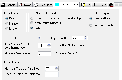
Figure 1 illuminates the maximum trials per time step. This number reflects the model's persistence in seeking convergence during dynamic wave routing. 🌐🔍
Convergence in the Dynamic Wave Solution:
- The dance of calculation continues until the steps match the maximum number of trials. 🕺💃
- At each time step, the flows and depths are reassessed. If all nodes agree within the head tolerance, the iteration halts. 👍
- A single non-convergent node increments the Non-Converge Count, a rare occurrence. 📊
- Efficiency tip: Links that can be bypassed are noted, speeding up the process when dynamic wave calculations are unnecessary. 🏎️💨
With SWMM 5, you're not just running a model; you're conducting an orchestra of data where each note is a time step, each rest a chance to converge, and the symphony is the fluid mechanics of urban water systems. 🎼🌆"
 |
| Figure 1. Maximum number of trials per time step |
In the dynamic world of SWMM 5, the Routing Time Step Summary serves as a crucial indicator of model stability and efficiency 🌐🔧. Here's a snapshot:
Percent Non-Converging: This is the fraction of time when at least one element in the model's intricate network didn't align within the set number of trials per step. It's the ratio of the total non-convergent steps to the overall number of steps taken during the simulation 🔍💡.
Dynamic Wave Solution Mechanics: Like a conductor leading an ensemble, the program meticulously iterates until the number of steps aligns with the maximum trials allowed. Each step is a note, each calculation a beat 🎶🧮.
Convergence: It's a delicate balance. If all node depths settle within the accepted variance (below the head tolerance) after more than one step, the model ceases iterations. Harmony is achieved ✅🔄.
Non-Convergence: However, should even a single node remain unresolved, the Non-Converge Count ticks up, a rare but noted event in the symphony of simulation 🚦📊.
Efficiency: Not every link needs a detailed calculation at each step. By identifying which can be bypassed, the program conserves energy, speeding up like a swift current bypassing a tranquil pool 🏎️💨.
Figure 2 likely illustrates this concept further, capturing the essence of a model that is both robust and refined. By understanding these dynamics, you can ensure a smoother, more accurate simulation, leading to more reliable predictions and planning in urban water systems 🌟🌊.
 |
| Figure 2. Link Bypass is based on the Upstream and Downstream Nodes |
while ( Steps < MaxTrials )
{
// --- execute a routing step & check for nodal convergence
initNodeStates();
findLinkFlows(tStep);
converged = findNodeDepths(tStep);
Steps++;
if ( Steps > 1 )
{
if ( converged ) break;
// --- check if link calculations can be skipped in next step
findBypassedLinks();
}
}
if ( !converged ) NonConvergeCount++;
// --- identify any capacity-limited conduits
findLimitedLinks();
return Steps;
Tuesday, December 30, 2014
How to Make a Trapezoidal Inflow Time Series in InfoSWMM
- . Use the Inflow Icon at a Node in the Attribute Browser
- . Use either an Inflow Time series with date/time/value or
- . A baseline flow value with a pattern
- . The time series comprise a Date that matches your simulation time period
- . A hour:minute:second Time value in the Time Series Table
- . A flow unit with the units used in the General Tab of Run Manager
- . This time series is entered in the Attribute Browser under Time Series in the Operation Tab
 |
| How to Make An Inflow Time Series at a Node in InfoSWMM |
Sunday, December 28, 2014
The EPA SWMM 5 code and the various versions of Visual Studio
 |
| Visual Studio Configuration Properties |
Friday, December 26, 2014
Thursday, December 25, 2014
How to Make Scatter Graphs in InfoSWMM and H2OMap SWMM
 |
| Figure 1. The Basic Velocity vs Depth Scatter Graph in InfoSWMM |
 |
| Figure 2. The Log/Log Options for a Scatter Graph. |