ScienceDaily (Dec. 1, 2010) — Rain gardens are increasingly popular with homeowners and municipalities and are mandatory for many communities nationally. U.S. Department of Agriculture (USDA) scientists are finding ways to improve rain gardens so they not only reduce runoff, but also keep toxic metals out of storm drains.
Autodesk Technologist with Information about Stormwater Management Model (SWMM) for watershed water quality, hydrology and hydraulics modelers (Note this blog is not associated with the EPA). You will find Blog Posts on the Subjects of SWMM5, ICM SWMM, ICM InfoWorks, InfoSWMM and InfoSewer.
Sunday, December 26, 2010
What is Link Bypass in SWMM 5?
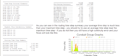
Time Step Critical Elements in SWMM 5
Pump Power Usage in SWMM 5
Friday, December 24, 2010
Non Linear Term in the Saint Venant Equation of SWMM 5
Wednesday, December 22, 2010
The number of Hydraulic Iterations in Various Versions of SWMM 5
Subject: The number of Hydraulic Iterations in Various Versions of SWMM 5.
The maximum number of iterations was 4 before SWMM 5.0.021 and 8 iterations after SWMM 5.0.021. In InfoSWMM and H2OMAP SWMM you can have a a minimum of 2 iterations or a maximum of 8 iterations for compatibility to SWMM 5 and backwards compatibly with your earlier InfoSWMM models.
.
Time Step Selection in SWMM 5
1st The time step you use in SWMM 5 is controlled from the top by the rainfall interval (Figure 1):
1. All of your time steps should be less than the rainfall interval,
2. The hydrology time step should be less than or equal to the smallest raingage rainfall interval in your network,
3. The hydraulic time step should be less than or equal to the hydrology time step and should be based on the hydraulic needs of the your network. Short length links, pump and weirs may require a smaller maximum hydraulic time step.
2nd The report time step controls what you see in the graphics output of SWMM 5. If you see a large difference between that you see in the graphics output and the report text file it is because you have a large difference between the report time step and the average time step used during the simulation.
Solution: If there is a large discrepancy in the graphics and report text file then the best solution is to reduce the maximum time hydraulic time step so it is closer to the average time step and also to make the report time step closer to the Maximum time step (Figure 2).
Figure 1: Relationship between the rainfall, hydrology and hydraulic time steps.
Figure 2: Relationship between the minimum, average and maximum simulation time steps and the report time step.
Tuesday, December 21, 2010
Pump Priorities in SWMM 5
Node Surcharge Summary in SWMM 5
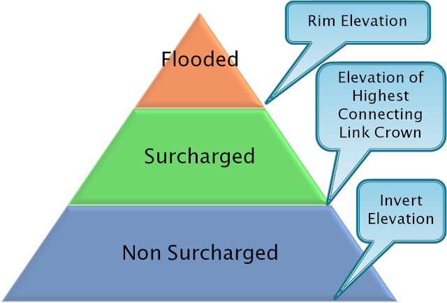
In SWMM 5 (Storm Water Management Model), surcharging refers to a condition where water levels rise above the highest point, or crown, of the conduits (pipes) in the drainage network. This situation usually occurs when the system's capacity is exceeded due to high levels of stormwater or wastewater inflow.
The SWMM 5 report file (RPT file) includes a Node Surcharge Summary Table, which provides crucial details about the duration and extent of these surcharging events.
Node Surcharging:
A node is a point in the network where pipes connect. Surcharging can occur at a node in the following conditions:
If the node cannot store additional water (i.e., it cannot 'pond') and the water depth at the node exceeds the crown elevation of the highest pipe connected to that node.
If the node can store additional water (it can 'pond'), surcharging occurs when the water depth exceeds the crown elevation of the highest pipe connected to the node but remains below the full depth of the node.
Essentially, surcharging happens when the system cannot accommodate the excess water, leading to water levels rising above the pipe's topmost part but not yet reaching the full depth of the node.
Node Flooding:
Node flooding is a more extreme event that occurs when the water surface level reaches or surpasses the rim elevation of the node. This situation means that the water is spilling out of the system, potentially leading to surface flooding.
Node Surcharge Summary Table (Figure 1)
This table in the RPT file presents a summary of the surcharging events at each node, including the duration of surcharging.
Definition of Surcharging at a Node (Figure 2)
This figure would typically show a diagram or explanation illustrating the conditions under which a node is considered to be surcharging, visually demonstrating the situations described above.
Definition of the Height above Crown and Depth below Rim (Figure 3)
This figure would likely provide definitions or illustrations explaining the 'Height above Crown' and 'Depth below Rim' columns in the Node Surcharge Summary Table. 'Height above Crown' refers to how much higher the water level is compared to the crown of the highest pipe, while 'Depth below Rim' refers to the difference between the water level and the full depth of the node.
These details allow engineers to understand the behavior of the drainage system under various flow conditions and inform necessary adjustments or improvements to manage stormwater effectively.
Monday, December 20, 2010
Swamee and Jain approximation to the Colebrook-White equation in SWMM 5
f = forcemain_getFricFactor(xsect.rBot, d/4.0, 1.0e12);
return sqrt(f/185.0) * pow(d, (1./6.));
double forcemain_getFricFactor(double e, double hrad, double re)
//// Input: e = roughness height (ft)
// hrad = hydraulic radius (ft)
// re = Reynolds number
// Output: returns a Darcy-Weisbach friction factor
// Purpose: computes the Darcy-Weisbach friction factor for a force main
// using the Swamee and Jain approximation to the Colebrook-White equation.
{ double f;
if ( re < 10.0 ) re = 10.0;
if ( re <= 2000.0 ) f = 64.0 / re;
else if ( re < 4000.0 )
{ f = forcemain_getFricFactor(e, hrad, 4000.0);
f = 0.032 + (f - 0.032) * ( re - 2000.0) / 2000.0; }
else { f = e/3.7/(4.0*hrad);
if ( re < 1.0e10 ) f += 5.74/pow(re, 0.9);
f = log10(f);
f = 0.25 / f / f; }
return f;}
From http://en.wikipedia.org/wiki/Darcy_friction_factor_formulae
http://www.swmm2000.com/profiles/blogs/swamee-and-jain-approximation
Saturday, December 18, 2010
Link Surcharging Definitions in SWMM 5
The report or RPT text output file of SWMM 5 contains a table that lists the Surcharged Conduits during the simulation (Figure 1).
The 5 columns in the table are:
- Hours Both Ends Surcharged
- Hours Upstream End Surcharged
- Hours Downstream End Surcharged
- Hours Above Full Normal Flow
- Hours Capacity Limited
Figure 1: The SWMM 5 Conduit Surcharge Table
Figure 2: The SWMM 5 Conduit Surcharge Table Definitions, the numbers in the 3rd column correspond to the columns in the Conduit Surcharge Table.
PID Control in SWMM 5 for an Orifice
PID Control in SWMM 5 for a Weir
; the PID controller adjusts the weir height to have a
; depth of 3 feet in Node 82309e
IF NODE 82309c DEPTH <> 3
THEN WEIR WEIR1@82309c-15009c SETTING = PID 10 -.01 -.01
; kp ki kd
PRIORITY 1
PID Control in SWMM 5 for a Type 3 Pump
Here is an example PID Rule that will keep the node depth at 3 feet in a SWMM 5 model.
RULE PID1
; the PID controller adjusts the flow in the pump to have a
; depth of 3 feet in Node 82309e
IF NODE 82309e DEPTH <> 3
THEN PUMP PUMP1@82309e-15009e SETTING = PID 10 -1 -1
; kp ki kd
PRIORITY 1
Figure 1: SWMM 5.0.021 Simulation Results
Figure 2: Source code for getPIDSetting in SWMM 5.0.021
Figure 3: Image source for the Block Diagram of a PID Controller Pid-feedback-nct-int-correct.png
Wednesday, December 15, 2010
Total Surcharge Time vs Total Time Above Rim Elevation in InfoSWMM
1. Total Surcharge Time is the total time above the crown of the highest connecting pipe to a node.
- A node is flooded if the node depth equals the node rim elevation – the flooded time is the total time excess flow coming out the top of the manhole,
- A node is flooded if the node depth is above the rim elevation and you are using the Surface Ponding Option – the flooded time is the ponding time
- A node is flooded if the node depth equals the node surchage elevation – the flooded time is the total time excess flow coming out the top of the surcharged manhole.

Tuesday, December 14, 2010
Monday, December 13, 2010
IBM helps the City of Corpus Christi get smarter
IBM helps the City of Corpus Christi get smarter
IBM’s Guru Banavar discusses how Corpus Christi is getting smarter by tracking the city’s assets. In order to keep the citizens happy, you have to manage the city’s assets.
Wellington E Webb, the former mayor of Denver, Colorado, once said: “The 19th century was a century of empires, the 20th century was a century of nation states. The 21st century will be a century of cities.”
...
That’s why the cities need to be smarter. And to do this, each part of the infrastructure needs to be more intelligent. This means the cities need to start collecting data on everything including streets, bridges, parks, buildings, fire hydrants, water mains and storm water ditches. Link HereSaturday, December 11, 2010
Calibration Concepts from Serendipity
Wednesday, December 8, 2010
How to Decide on a Time Step in InfoSWMM
Note: How to Decide on a Time Step in InfoSWMM
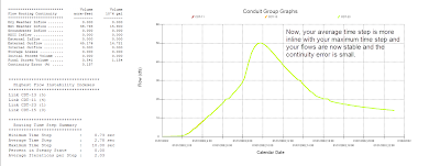
Step 1: Your first guess was 300 seconds which had a very large continuity and unstable links. If you look at the your average time step a good time step would be 10 seconds based on your average time step of 2.6 seconds.

Step 2: Run your model with a time step of 10 seconds and check the flows and the continuity error. In this case by using a maximum time step near the average time step you got rid of the continuity error and the unstable link flows.

Tuesday, December 7, 2010
Export from WeatherUnderground using the CSV File Export Option to InfoSWMM
Weather Underground is a site that provides excellent local weather information in the form of graphs, tables and csv files. You can use the data very easily in InfoSWMM by copying from Excel to a time series in InfoSWMM. Here is the rainfall for a storm event in Tampa, Florida in September 11, 2010
Step 1: Export from WeatherUnderground using the CSV File Export Option
Step 2: The data imported from the csv file to Excel and after the text to columns tool is used looks like this in Excel. The data is now ready to be imported into InfoSWMM after the time column is adjusted to fall on even 5 minute intervals. In Excel you can use the formula @ROUND((B2)/"0:05:00",0)*"0:05:00" to round all of the time values to 5 minutes. If you do not do this step then you will have problems in InfoSWMM due to the rainfall interval not being equal to the defined raingage interval.
Step 3: You will need to format the new rounded time as a time format for import into a InfoSWMM time series. The time series is created in the operation tab of the attribute browser.
Step 4: Open up and make a new time series in InfoSWMM.
Step 5: Copy and then paste the date, rounded time column and rainfall column into the InfoSWMM time series columns.
Step 6: Make a raingage in the DB Table in InfoSWMM that will use the time series you just made. In the case of the Weather Underground data we will use inches, intensity, a rainfall interval of 5 minutes, time series and the name of the time series. SCF should be 1 for Snow conversion and do not need to include a Filename or Station name as we are not using an external file.
Flow Units In InfoSWMM may be different then the Output Link Flow Units
The flows units selected in Run Manager determines the flow units of all incoming units including DWF, Inflow Time Series and other features in pump curves and other curves. The output unit manager determines what you see when you make a graph of the link flow. For example, you can have dry weather inflow of CFS and output units of GPM or MGD if you so request and set the correct flags in the interface.
Hysteresis Effect in the Link Flow versus Depth Relationship in SWMM 5
You can often get a hysteresis effect for the Flow versus Depth relationship in SWMM 5 due to the five component St. Venant equation used to simulate the flows (http://swmm5.blogspot.com/2010/12/what-are-units-for-five-st-venant-flow.html) . A hysteresis effect is having two or more flow values for the same depth value in the link. For example, this image shows how the link 8100 has a different flow for the same depth in the rising and falling limb’s of the hydrograph. This is due to the different values for the upstream and downstream head, hydraulic radius and cross sectional area during the falling and rising hydrograph, respectively.
Monday, December 6, 2010
How is RHO computed for a Link in SWMM 5?
SWMM 5 uses a sliding metric to calculate the cross sectional area and hydraulic radius used in the simulation for the link dynamic flow. The area and hydraulic radius used moves from the Upstream End of the Link to the Midpoint of the Link based on the Froude number and a few other considerations (see Figure 1 for the other considerations).
The area and hydraulic radius used as a function of the Froude Number:
1. Upstream cross sectional area and upstream hydraulic radius is used when the Froude Number > 1
2. Midpoint sectional area and hydraulic radius is used then the Froude Number is < 0.5
3. An area and hydraulic radius between the upstream and midpoint sections is used then the Froude Number is between 0.5 and 1
Figure 1: How to compute RHO based on the Froude Number.
Figure 2: The computed value of the Froude Number and the value of RHO over time.
Figure 3: Relationship between the upstream area, midpoint area and the actual area used during the simulation.
Sunday, December 5, 2010
What are the Units for the five St. Venant Flow Terms in SWMM 5 and InfoSWMM?
This is how the flow is calculated in a link in InfoSWMM. It uses the
· Upstream and downstream head,
· The user input length,
· The weighted cross sectional area and hydraulic radius as I explained in the previous email,
· The Center velocity,
· The Center Cross sectional area, and
· The Upstream and Downstream Cross sectional area.
The slope as listed in the output file is more for reference and is actually not used in the St. Venant Solution. The way the program usually works is that the friction slope lags the water surface head slope with the difference made up by the change in flow. The two non linear terms are usually small and only affect the flow during reverse or backwater events.
The new flow (Q) calculated at during each iteration of time step as
(1)Q for the new iteration = (Q at the Old Time Step – DQ2 + DQ3 + DQ4 ) / ( 1.0 + DQ1 + DQ5)
In which DQ2, DQ3 and DQ4 all have units of flow (note internally SWMM 5 has units of CFS and the flows are converted to the user units in the output file, graphs and tables of SWMM 5).
The equations and units for DQ2, DQ3 and DQ4 are:
(2)Units of DQ2 = DT * GRAVITY * aWtd * ( H2 – H1) / Length = second * feet/second^2 * feet^2 * feet / feet = feet^3/second = CFS
(3)Units of DQ3 = 2 * Velocity * ( aMid – aOld) * Sigma = feet/second * feet^2 = feet^3/second = CFS
(4)Units of DQ4 = DT * Velocity * Velocity * ( aDownstream – aUpstream) * Sigma / Length = second * feet/second * feet/second * feet^2 / feet = feet^3/second = CFS
The equations and units for DQ1 and DQ5 are:
(5)Units of DQ1 = DT * GRAVITY * (n/PHI)^2 * Velocity / Hydraulic Radius^1.333 = second * feet/second^2 * second^2 * feet^1/3 * feet/second / feet^1.33 = Dimensionless
(6)Units of DQ5 = K * Q / Area / 2 / Length * DT = feet^3/second * 1/feet^2 * 1/feet * second = Dimensionless
The five components calculated at the each time step and at each iteration during a time step and together predict the new Link Flow (Q) in SWMM 5. The value of the different components can be seen over time in Figure 1 and as a component percentage in Figure 2 and 3.
Figure 1: The Five St. Venant Components over time.
Figure 2: The relative magnitude of the St Venant terms over time for the same for the same link as in Figure 1.
Figure 3: The relative magnitude of the St Venant terms over time for the same for the same link as in Figure 1 shown in an area chart normalized to 100 percent. Normally the DQ1 and DQ2 terms balance each other except for backwater conditions or reverse flow in which the terms DQ3 and DQ4 can dominate.
Thursday, December 2, 2010
Rain Gardens Are Sprouting Up Everywhere - Science Daily
Rain Gardens Are Sprouting Up Everywhere
The Goal of SWMM5 Input Files
🌟 SWMM5 (Storm Water Management Model 5) is a widely used urban hydrology and hydraulic modeling software developed by the United States E...
-
@Innovyze User forum where you can ask questions about our Water and Wastewater Products http://t.co/dwgCOo3fSP pic.twitter.com/R0QKG2dv...
-
Subject: Detention Basin Basics in SWMM 5 What are the basic elements of a detention pond in SWMM 5? They are common in our back...
-
Engine Error Number Description ERROR 101: memory allocation error. ...